The Telco Energy Portfolio: How Operators Buy, Hedge and Save Electricity

The article in three minutes

For readers who want the argument before the detail, these are the ten ideas the rest of the article develops.

1. A telco’s electricity is a portfolio, not a purchase. Volume, timing, price risk and the full bill have to be managed together.
2. The network has a continuous base load. It varies with traffic, temperature and technology, but it never stops — including in the evening and night hours that solar cannot cover.
3. Wholesale prices are set by the last plant needed in each hour. In many hours that is a gas plant, so gas, weather and conflicts move the price of all electricity in those hours; in others, renewables, hydro, nuclear, imports or batteries do.
4. The energy price is less than half of the bill. Network tariffs, system charges, levies and taxes are not protected by any energy contract.
5. A cheap PPA is not cheap electricity. A 35 €/MWh solar contract can cost 85 €/MWh once it serves a load that also consumes at night.
6. Hedging buys time, not immunity. It decides how much of a shock reaches the P&L and when; a lasting price rise eventually reaches every contract.
7. Portfolios should be chosen on cost and risk together. In a simple example, flat and diversified portfolios cut the cost in a crisis year by more than a third against buying at market prices.
8. The hedge cliff is the decision of the decade. Long-term contracts signed before 2022 are expiring; renewing late and all at once resets the cost base at the worst moment.
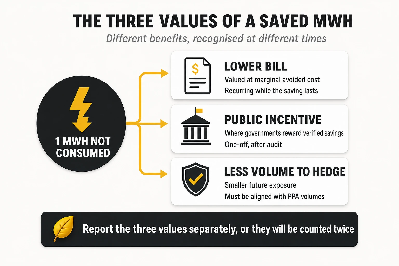
9. Saving energy is worth what the contract lets you avoid. The same switched-off MWh has a different value under a spot contract, a financial hedge or a physical PPA.
10. Anticipation is a policy. Signals and thresholds should trigger a disciplined review within agreed limits — not automatic purchases, and not improvisation.

1. A network that never sleeps, buying from a market that changes by the hour

Telecom operators consumed about 300 TWh of electricity in 2024, roughly 1% of global electricity use, and spent around 50 billion dollars on energy, according to the GSMA Mobile Net Zero 2026 report. Energy is not the largest cost of an operator — site rentals and labour usually rank ahead of it — but it is the one whose unit price can triple in a single quarter.

That is what happened in 2022. In the third quarter of that year, the CEO of Telia described a “tripling of energy prices in the quarter” while the company was about 70% hedged, and raised its full-year energy cost increase to roughly SEK 900 million (Mobile World Live). Moody’s estimated that European operators were, on average, about two-thirds hedged for 2022, with that protection unwinding from 2023 (Light Reading). ING expected the sector’s energy costs to at least double in 2023, partly because many operators had locked 2023 volumes at crisis prices (ING Think).

Four years later, the same question is back. In October 2026, the benchmark European gas price traded at around 86 €/MWh, close to its highest level since December 2022, with EU gas storage well below its five-year average going into winter. And the contracts that protected many operators in 2022 — long-term renewable power purchase agreements signed in the late 2010s at prices that now look very low — are approaching the end of their terms.

The thesis of this article is that electricity in a telco has become a portfolio management problem, not a purchasing problem. It has four dimensions that must be managed together:

• Volume: how much the network consumes, and how decommissioning, modernisation and growth will change it over the next ten years.
• Shape: when it consumes. A network draws power 24 hours a day, while the generation with the lowest running cost — solar above all — produces for only part of it.
• Price risk: how much of that consumption is protected, at what price, for how long, and what happens when the protection expires.
• The full bill: network tariffs, system charges, levies and taxes that no energy contract covers.

Behind all four sit forces the operator does not control: weather, which moves prices every day; wars and supply shocks, which can reset the price level for years; and policy, which changes the rules and the charges. The operator cannot forecast them. It can decide in advance how much of each shock reaches its P&L, and what it will do when the warning signs appear.

How to read this article

The article is written for readers who know telecoms but not electricity markets, and moves from mechanisms to decisions. Sections 2 to 6 explain the load, the market, what moves prices, what to watch and what the bill contains. Sections 7 to 9 cover the instruments, how to choose a portfolio and how a contract actually runs. Sections 10 and 11 deal with consumption and the value of saving it. Sections 12 and 13 review what operators are doing. Sections 14 to 16 turn all of it into an operating model, strategic options and a playbook. Section 17 concludes.

2. How much electricity a telco uses, and where it goes

The starting point of any energy strategy is the load itself: large, spread over tens of thousands of small sites, and never switched off.

The size of the load

The GSMA Mobile Net Zero 2026 report (data year 2024) gives the order of magnitude. Operators consumed about 300 TWh — 43% in Greater China, 17% in the rest of Asia Pacific, 13% in North America, 11% in Europe — or about 29 kWh per connection, from 58 kWh in North America to 7 kWh in Sub-Saharan Africa. They also burned about 2.5 billion litres of diesel and gasoline, at an estimated 3 billion dollars, plus some 900 million litres at tower companies; in some countries diesel accounts for up to half of operating costs. Renewables covered 24% of their electricity, up from 10% in 2019, with Europe at about 70% and Greater China at 6%. At company level, Deutsche Telekom reported 11,053 GWh of group consumption in 2024, down from 12,270 GWh in 2021 (Deutsche Telekom).

Where the electricity goes

Access networks dominate. Disclosures from more than 30 operators analysed by the GSMA show that about three-quarters of electricity is used in fixed and mobile access networks, while data centres are below 10% of total use except in operators with large data centre businesses, mainly in Asia. GSMA Intelligence has estimated that the radio access network alone uses on average 73% of a mobile operator’s energy (Light Reading).

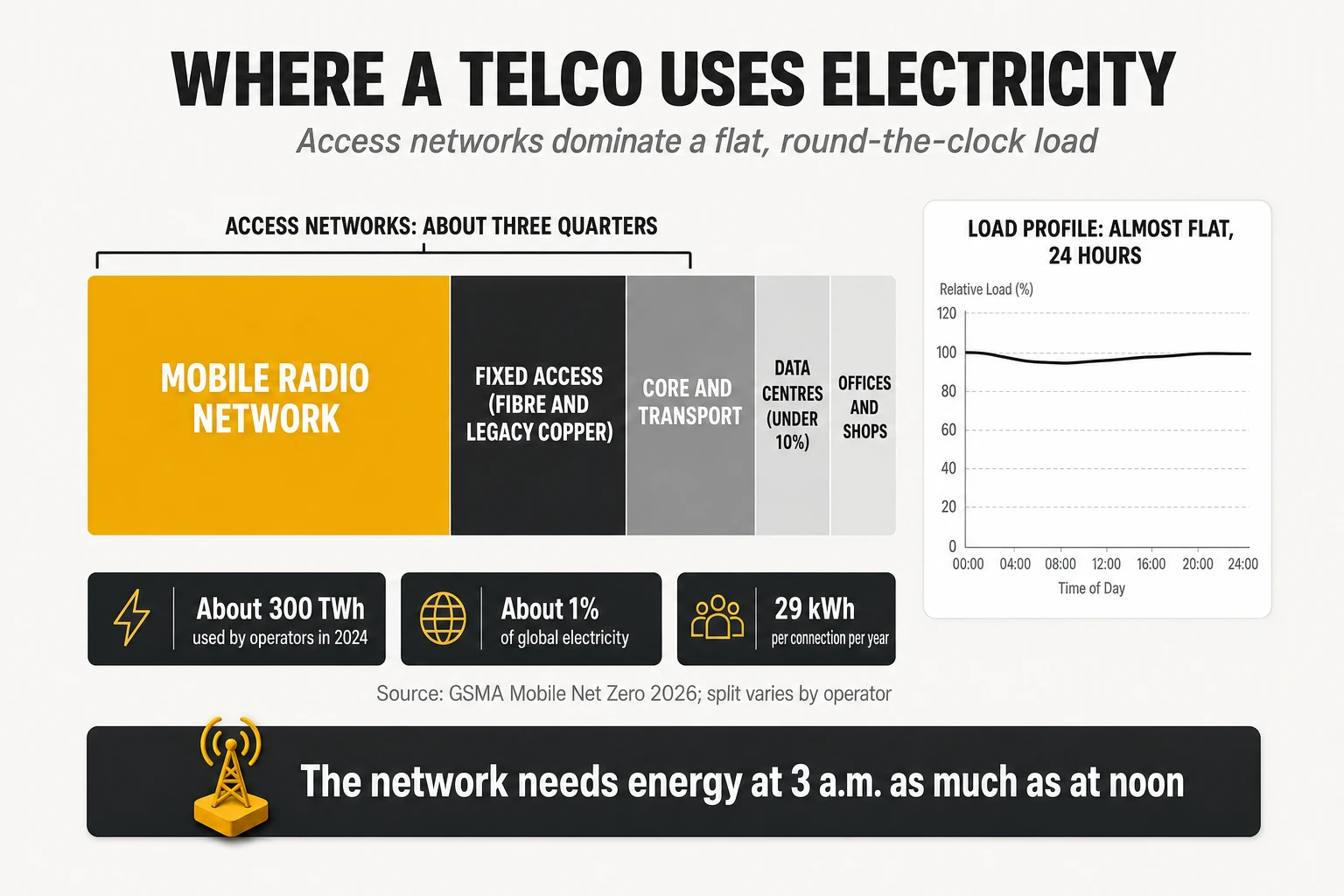
A typical integrated operator’s consumption can be split into five blocks, each with a different trajectory:

• Mobile network: the largest block, growing with 5G densification and traffic, but with strong efficiency levers (sleep modes, 3G sunset, modern radios).
• Modern fixed network: fibre access, aggregation and IP transport; relatively efficient per line and growing slowly.
• Legacy fixed network: copper exchanges, PSTN, old transport. A large share of consumption for a small and shrinking share of traffic — the main target of decommissioning.
• Data centres and hosting: stable or growing, and in some operators growing quickly with AI and cloud.
• Offices, shops and other buildings: a minor share, often managed separately.

A continuous base load, with variations

Network consumption never stops, but it is not perfectly flat. A large part of the equipment — power supplies, transport, core platforms, base station hardware without advanced sleep features — draws nearly the same power whether it carries traffic or not, which creates a continuous base load. On top of it, consumption varies with traffic (lower at night, more so where radio sleep modes are active), with temperature (cooling works harder in summer and in the afternoon) and with technology (newer equipment scales its consumption with load better). For procurement, the essential fact is the base: a telco needs a large amount of energy at 3 a.m. on a windless January night, when cheap solar is absent and prices can be high. In the examples of this article, that load is simplified as flat.

A fixed broadband line consumes about 50 kWh a year in the network and a mobile broadband connection about 25 kWh, according to the GSMA, with customer premises equipment adding about 80 kWh per line that is not included in operators’ totals. Those numbers explain why fibre migration and legacy switch-off are energy projects as much as network projects.

How much of the cost base is energy

The share of energy in operating costs is often quoted and rarely sourced. Figures of 20-40% of network opex circulate widely, mostly from vendor material; Moody’s put energy at about 5% of operators’ total opex in 2022 (Light Reading), and ING at about 2% of total costs including depreciation (ING Think). The ranges are not contradictory; they use different denominators. Energy is a mid-sized line in a European operator’s total cost base, a large share of network opex, and — in markets that depend on diesel — one of the biggest costs of all.

What makes it strategic is not its size but its volatility. In 2022, KPN expected 50-60 million euros of additional energy costs for 2023 despite having cut its absolute energy use by 45% since 2010 (KPN), and analysts estimated that Vodafone, hedged at about 85% for its financial year 2023, could face around 400 million euros of additional cost per year if spot prices held (Light Reading).

3. How electricity is produced, traded and priced

An operator does not buy electrons from a specific power plant. Its exchanges, base stations and data centres take electricity from the grid, which carries a physical mix of whatever is generating at that moment: solar, wind, hydro, nuclear, gas, coal, biomass. What the operator buys is a commercial and financial position — a contract that defines how much it pays for a volume of energy over a period, who absorbs the deviations, and which environmental attributes come with it. That separation between physical flow and financial contract is the first thing to understand.

The five players in any power system

Every liberalised electricity system has the same five roles, whatever their local names. Generators produce and sell electricity. The market operator runs the exchanges where energy is traded for the next day and within the day. The system operator balances generation and consumption second by second and buys the reserves that keep the grid stable, passing the cost to consumers. Transmission and distribution networks carry the energy and are paid through regulated tariffs. Retailers buy energy, schedule it, absorb or pass through imbalances, manage thousands of metering points and send the invoice. A large telco deals with all five, and each is a separate lever.

The merit order: why the most expensive plant sets the price for everyone

Most wholesale electricity markets clear with marginal pricing. For each trading period (an hour, or since October 2025 a quarter of an hour in the coupled European day-ahead market (European Commission)), generators submit offers and buyers submit bids. The algorithm accepts offers from the cheapest upwards until demand is met. The last offer needed — the marginal unit — sets the clearing price, and every accepted generator receives that price, whatever it offered.

Generators offer at roughly their variable cost, which explains the order of the stack: solar and wind close to zero (or below, when subsidies are paid per MWh produced), then nuclear and run-of-river hydro, then coal and gas at the cost of fuel plus carbon; reservoir hydro offers at the opportunity cost of its water.

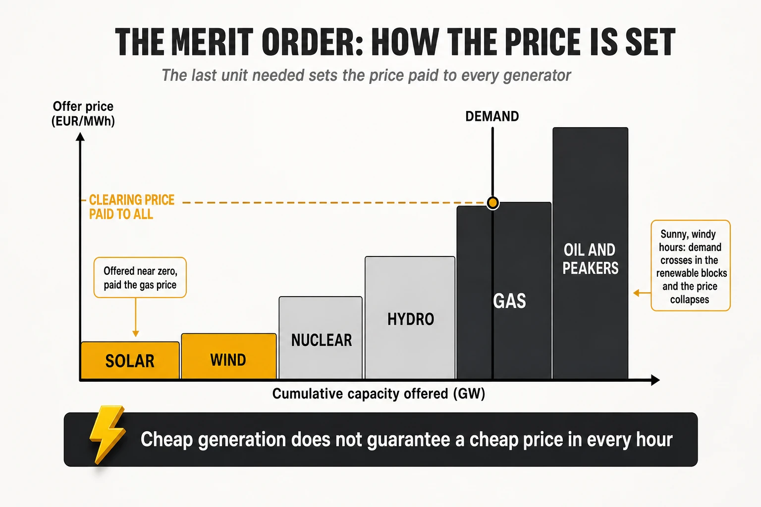
The consequence surprised many buyers in 2022. When the demand curve crosses the stack in the segment occupied by gas plants, the price of electricity is set by the cost of gas, even if most of the energy in that hour came from cheap renewables and nuclear. A sharp rise in gas prices is then passed almost entirely to the price of all electricity in those hours. When the stack is crossed in the renewable segment — a sunny, windy spring afternoon — the price can collapse to zero or turn negative.

It is wrong to say that gas always sets the price. How often it does depends on the generation mix and the hour. A study by the European Commission’s Joint Research Centre found that gas plants set the EU price about 55% of the time in 2022 while producing roughly 19% of the electricity; an IEEFA analysis published in April 2026 estimates that in most EU markets gas now sets the marginal price for a few hundred to about 1,500 hours a year, with much higher shares in Italy and lower ones in markets dominated by nuclear, hydro or solar. The methods differ, so the honest reading is a range, not a number. The direction is clear, though: the more renewable capacity a system has, the more hours are priced near zero, and the more the remaining hours — evenings, nights, windless winter weeks — are priced by flexible resources, of which gas is still the most common in Europe and much of the world. For a buyer with a continuous 24-hour load, that spread between cheap and expensive hours is the core of the problem.

Not every market works the same way

The marginal pricing logic is common, but the market architecture varies by region, and it changes what a telco can buy.

Market model	Where	How the price is formed	What it means for a telco
Zonal day-ahead and intraday markets	European Union, Norway, UK (own design), Japan (JEPX), India (power exchanges for a share of volume)	One price per bidding zone and period, set by marginal pricing across coupled exchanges	Hedging with standard forwards is easy; PPAs settle against a zonal price that is the same for all sites in the zone
Nodal markets run by an ISO	Most of the United States (ERCOT, PJM, CAISO, MISO, NYISO), New Zealand, Singapore (uniform price from nodal)	Locational marginal prices that differ by node because of congestion and losses	A virtual PPA settles at the project’s node, while sites consume at other nodes: basis risk appears
Gross pool with regional prices	Australia (NEM)	Five regional prices, very high caps and floors, five-minute settlement	Extreme volatility; caps, swaps and PPAs are standard tools for large buyers
Regulated or single-buyer systems	Much of Africa, the Middle East, parts of Asia and Latin America	Tariffs set by the regulator or the state utility; limited or no retail choice	Procurement is about tariffs, captive generation and diesel replacement, not hedging; open-access or wheeling rules decide whether PPAs are possible

Caption: Wholesale market architectures by region. The procurement toolbox described in this article applies fully to liberalised markets and only partially to regulated ones.

The practical difference is large. A European operator can lock prices three or four years ahead with standard forwards; a US operator signing a virtual PPA must model the price gap between the plant’s node and its own load; an operator facing a single state utility can only work on tariffs, on-site generation and efficiency.

Each technology: what it costs, when it produces, what it does to the price

A telco buyer does not need to become a power-plant engineer, but it needs to know which technology drives which risk, and how each one can — or cannot — be used to build a supply portfolio. The table summarises the general pattern; the weights change from market to market.

Technology	Variable cost	When it produces	Typical effect on price	What it means for a 24/7 buyer
Solar PV	Near zero	Daylight hours, more in summer	Depresses midday prices, sometimes below zero; adds nothing at night	Often the lowest PPA price in sunny markets, but the weakest hourly match for a flat load
Onshore and offshore wind	Near zero	Day and night, weather-dependent, seasonal	Lowers prices when it blows; cannot be guaranteed for any hour	Usually a better hourly fit than solar, but site-specific; can fail for days
Run-of-river hydro	Near zero	Follows river flows; little ability to shift	Behaves like other variable renewables	Rarely contractable on its own
Reservoir hydro	Opportunity cost of water	Dispatchable within hydrological and environmental limits	Offers close to the price of the alternative it displaces; dry years raise prices	A key driver to watch, not a product to buy
Pumped storage	Cost of pumping plus losses	Pumps at cheap hours, generates at expensive ones	Narrows the daily spread	Storage, not a net source of energy
Nuclear	Low	Flat, except refuelling and outages	Stabilises prices; long outages raise them	Underpins baseload products; outage calendars and closures matter
Gas combined cycle	Fuel plus carbon	Flexible, fills the gaps left by others	Sets the price in many evening, night and winter hours, but not all	The main transmission channel of fuel and geopolitical shocks
Coal and lignite	Fuel plus high carbon cost	Flexible, declining	Expensive where carbon is priced	Closures remove flexibility and can raise peaks
Batteries	Charging cost plus losses and degradation	Two to four hours of discharge after charging	Compress the evening peak; increasingly set the price in some markets	Improve the shape of solar contracts; do not cover multi-day shortfalls
Interconnections	Price of the neighbouring market	Whenever there is spare capacity and a price gap	Import cheaper power, export surpluses; congestion splits prices	Determine how much a regional shock reaches the local price

Caption: How each technology influences wholesale prices and what it implies for a buyer with a round-the-clock load. General pattern; local conditions can change it.

A technology that moves the market is not necessarily a product the buyer can contract. A telco can sign PPAs with solar or wind plants, buy hybrid products with storage, or buy baseload and fixed-price products from utilities; it does not usually contract hydro, nuclear or gas output directly. The technologies matter because they explain the price of whatever product the buyer does buy, and the hours when that product is cheap or expensive.

Solar: four prices that are often confused

When a buyer hears that “solar costs 35 €/MWh”, four different numbers may be meant: the generation cost of building and running the plant; the capture price, the average market price the plant actually earns in its production hours; the PPA price agreed in a contract, which reflects the generator’s expectation of future capture prices plus its financing needs; and the effective cost for the buyer, which adds the energy bought when the plant does not produce and subtracts the resale value of its surpluses. In markets with a lot of solar, the capture price falls well below the average: in Germany, solar plants captured just under 55 €/MWh in 2025 (S&P Global) against an average day-ahead price of about 90 €/MWh (Electricity Maps). Only the effective cost matters to a telco; section 7 shows how far it can be from the headline.

Wind: complementary, but not always

Wind often blows at night and in winter, when solar is weak, so the two combined are smoother than either alone — but not always. Calm, overcast winter weeks (Dunkelflaute, “dark doldrums”) reduce both at once, usually when demand is high. On 12 December 2024, the German day-ahead price reached 936 €/MWh for one hour, against an average of about 79 €/MWh for the year; regulators attributed the spikes to low wind and solar output during high demand, and found that imports prevented even higher prices (SMARD / Bundesnetzagentur). Mixing wind and solar reduces hourly exposure on average; it does not remove the tail risk.

Hydro: three different economics

• Run-of-river plants follow river flows and cannot store water; they behave like variable renewables.
• Reservoir plants choose when to release water, within technical, hydrological and environmental limits, and offer at the opportunity cost of using it now — roughly the price of the alternative it replaces. Full reservoirs lower prices mostly by displacing gas in expensive hours.
• Pumped storage pumps water uphill at cheap hours and returns part of it at expensive hours: storage with losses, not a net source of energy.

Reservoir levels alone do not tell the buyer what will happen to the price. What matters is usable energy and when it will be released: water stored in spring may be committed to irrigation in summer, while a dry year in a hydro-heavy system can raise prices for months.

Nuclear, batteries and interconnections

• Nuclear produces a flat output at low variable cost and underpins baseload products. A buyer rarely contracts it directly: it buys a baseload product priced at the market’s expectation, not at the plant’s cost. Its risks reach the buyer indirectly, through long outages, heatwave output cuts and closures.
• Batteries shift energy in time; they do not produce it. Their value depends on duration (usually two to four hours), round-trip losses (typically 10-15%), degradation and the price spread they arbitrage. They compress the evening peak and improve solar contracts, but cannot cover a week of low wind — and as fleets grow, spreads narrow: in Australia they fell 85% in a year (AEMO data via PV Tech).
• Interconnections let power flow between markets when there is spare capacity and a price gap. Uncongested, neighbouring markets converge and share shortages; congested, prices split, and a poorly connected market — an island system, or a region with few cross-border lines — can decouple for better or worse. Interconnection capacity decides how much a neighbour’s shock reaches the local bill.

The diagnosis for a telco is simple. The technologies with the lowest variable cost produce during only part of the day or the year, while the network consumes around the clock. The hours that solar cannot cover — evenings, nights, winter, calm weeks — are priced by whichever flexible resource is marginal: often gas, sometimes hydro, imports or, increasingly, batteries. Every procurement decision should be judged by how it handles that mismatch.

4. What moves the price: weather, conflicts and policy

Electricity prices move for three families of reasons, and a telco cannot control any of them. Weather changes how much energy is demanded and how much cheap generation is available. Geopolitical events change the price and availability of the fuels that set the price in the hours renewables cannot cover. Policy and regulation change the rules, the taxes and the costs added on top. What the operator can control is how much of each shock reaches its P&L, and when.

Weather: the variable that moves prices every day

Weather is the most frequent driver of electricity prices, and its effect is felt within hours. It acts on both sides of the market at the same time.

Weather event	What happens in the market	What happens to a telco
Cold spell	Heating demand rises; in winter, solar is weak and wind is not guaranteed	Spot and intraday prices spike; unhedged night-time volume is exposed
Heatwave	Cooling demand rises; thermal and nuclear plants may have to reduce output when river water is too warm	Prices rise in the evening, and the network’s own cooling consumption rises at the same time
Calm, overcast week (Dunkelflaute)	Wind and solar output collapse together; flexible plants, storage and imports set the price	Short but extreme price peaks — 936 €/MWh in Germany on 12 December 2024
Drought	Reservoir hydro is reduced for months; gas fills the gap	Higher prices over a whole season, in hydro-dependent systems
Wet, windy year	Abundant hydro and wind displace gas	Lower prices; hedges signed earlier look expensive in comparison
Sunny spring	Solar floods midday hours, often with low demand	Zero or negative prices at midday; solar PPAs capture less

Caption: How weather moves electricity prices and how each event reaches a telco’s bill.

Weather can amplify a geopolitical shock. In 2022, drought and heatwaves in France came on top of corrosion problems in the nuclear fleet: nuclear output fell to its lowest level since 1988 and hydro to its lowest since 1976 (RTE). France had to import, and the pressure spread across Europe just as gas was at record levels.

For a telco, weather has a double effect that is easy to miss. A heatwave raises the market price and, at the same time, the operator’s own consumption, because cooling systems in exchanges, data centres and cabinets work harder. The volume exposed to high prices grows precisely when prices are high.

Conflicts and geopolitics: the shocks that reset the price level

Weather moves prices for days or seasons; geopolitical shocks can change the price level for years. They mostly travel through fuel markets — gas, LNG, oil and coal — and reach electricity only in the hours when fossil plants are marginal. How much of a gas shock appears in the power price therefore depends on how often gas sets the price in that market; how much reaches a telco depends, in addition, on how much of its volume is already hedged.

• 2022: the invasion of Ukraine. Russian pipeline gas, which had covered a large share of European supply, was progressively cut. The Dutch TTF front-month contract closed at about 221 €/MWh on 15 August 2022, an all-time high at that point, above the previous peak set right after the invasion in March (S&P Global). Power prices rose sharply in the hours when gas was marginal, and with them the bills of buyers exposed to the market: GSMA Intelligence estimated that operators’ energy costs rose between two and eight times, depending on the market and the hedge position (Light Reading).
• 2026: the Middle East and the Strait of Hormuz. After the strikes on Iran at the end of February 2026 and the disruption of shipping through Hormuz, LNG supply from the Middle East fell sharply. TTF, which had averaged under 45 €/MWh in June, passed 80 €/MWh in September (GMK Center) and traded around 86 €/MWh in mid-October, with EU storage at about 74% against a five-year average of around 86% (ING/OilPrice data). Oil followed: in April 2026 crude was more than 70% above its 2025 average, which hit operators that still rely on diesel at off-grid sites (GSMA Mobile Net Zero 2026).
• Sanctions and trade rules. The EU ban on Russian LNG from 1 January 2027 removes another source of supply in a tight market; tariffs and export restrictions on solar panels, batteries and critical minerals raise the cost of new renewable capacity and therefore of new PPAs.

The lesson for a buyer is that geopolitical shocks cannot be forecast, but exposure to them can be measured. The question is not “will there be a crisis?” but “if gas doubles next quarter, how many millions does our bill move, and how long until our hedges run out?”

Policy and regulation: the rules change too

Governments respond to price crises, and their responses change the economics of every contract. In 2022, European governments capped the price of gas used for power generation in some countries, subsidised consumers, and set an EU-wide emergency cap of 180 €/MWh on the market revenues of low-cost generators (Council Regulation (EU) 2022/1854). Such measures lower spot prices for unhedged buyers but bring their own charges and can change the value of existing hedges. Beyond crises, carbon pricing, periodic reviews of network tariffs, windfall taxes that trigger change-in-law clauses, and long-term market design — capacity mechanisms, nuclear extensions or closures, renewable auctions, the 2024 EU reform promoting PPAs — all move the cost of electricity for a decade at a time.

How a shock travels to the operator’s bill

A shock does not reach the P&L all at once; it travels through the operator’s contracts with different delays.

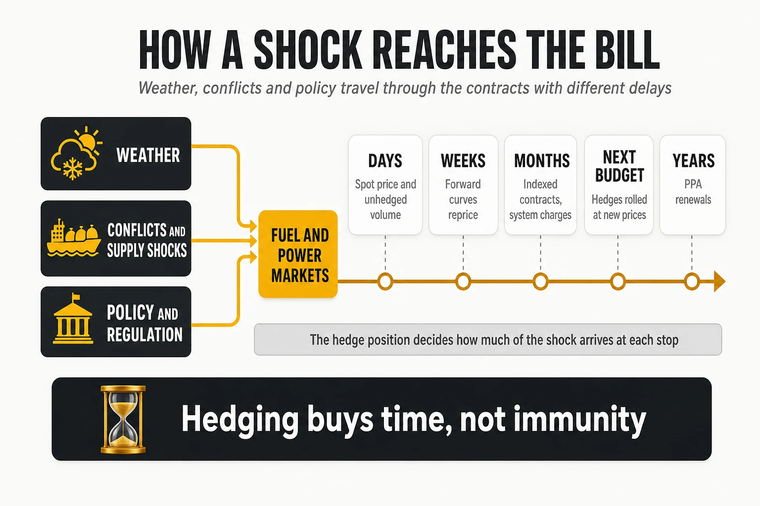
• Days: the spot price reacts, and with it the unhedged volume and any contract indexed to the day-ahead market.
• Weeks: forward curves reprice; any tranche bought now is bought at the new level.
• Months: retailers update fixed-price offers, system charges rise, the year-end estimate moves.
• Next budget: next year’s hedges are rolled at the new forward prices; a crisis absorbed this year arrives a year later.
• Years: long-term contracts are renewed at prices that reflect the new market; a shock lasting more than two or three years ends up in the whole portfolio.

This is why hedging buys time, not immunity. A well-hedged operator gains one to three years to adjust — to cut consumption, renegotiate, diversify supply — before a lasting price increase reaches its full cost base. Section 16 describes how to use that time.

5. The dashboard of an energy buyer: what to watch and why

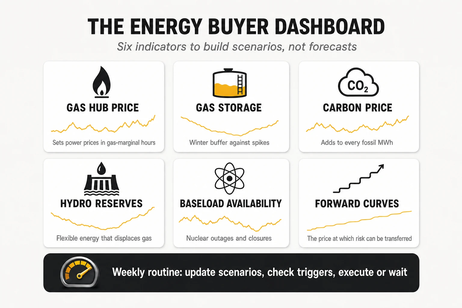
A telco energy team that only looks at its own invoices is driving by the rear-view mirror. The cost of next year’s unhedged volume, and the price of the hedges it will sign this quarter, are decided by a set of market indicators that translate the drivers of the previous section into numbers. None of them predicts the price mechanically. Together they tell the buyer which scenario is becoming more likely, and therefore when to accelerate or slow down purchases.

Six structural indicators: the price level for the coming months and years

• Gas price at the reference hub. TTF in continental Europe, NBP in Britain, Henry Hub in the United States, JKM for Asian LNG. In systems where gas is often marginal, it is one of the strongest drivers of power prices in the evening and night hours that matter for a 24/7 load.
• Gas storage levels. In Europe, the fill level of underground storage going into winter is the buffer against cold spells and supply disruptions. A low fill in October means more exposure to winter price spikes (daily data in GIE AGSI).
• Carbon price. The EU Emissions Trading System allowance (EUA) adds to the cost of every MWh produced from gas and coal; similar schemes exist in the UK, California and several Asian markets.
• Hydro reserves and rainfall. In systems with significant reservoir hydro, the usable water stored — not just the reservoir level — determines how much flexible, gas-displacing generation is available in the coming months.
• Availability of baseload plants. Nuclear outages and refuelling calendars, and coal or nuclear closures, remove low-cost energy from the stack.
• Forward curves. The prices at which next month, next quarter and the next three calendar years trade today. They are not forecasts, but they are the prices at which risk can actually be transferred, and every hedge decision is made against them.

Four short-term signals: what will happen in the next days and weeks

Structural indicators explain the price level; short-term signals explain the daily and weekly swings. They matter for operators with indexed or unhedged volume, for flexibility programmes and for timing tranches.

• Renewable output forecasts. Expected wind and solar production for the next days. A forecast of a calm, cloudy week in winter is the best early warning of price spikes.
• Demand forecasts and temperature. Cold and hot spells raise demand; holidays and mild weather lower it.
• Interconnection flows and outages. Available cross-border capacity, planned maintenance on interconnectors and congestion between price zones decide how much a neighbour’s surplus or scarcity reaches the local price.
• Regional gas hubs and LNG. TTF is the European benchmark, but plants in each country buy gas delivered into their own system. Regional hubs — THE in Germany, PEG in France, PSV in Italy, among others — can trade at a premium or discount to TTF depending on LNG arrivals, regasification capacity and pipeline links. In LNG-dependent systems, cargo arrivals and the spread to Asian prices (JKM) are a leading indicator.

Most of this data is public: in Europe, the ENTSO-E transparency platform, system operators and power exchanges publish forecasts, capacities, outages and prices, enough for a small team to build a useful dashboard.

From the gas price to the power price: a worked example

The link between gas and electricity can be estimated with simple arithmetic. A modern combined-cycle gas turbine converts about 55% of the energy in the gas into electricity. To produce one megawatt-hour of electricity it therefore burns about 1.82 MWh of gas.

With gas at 85 €/MWh, the fuel cost alone of that MWh of electricity is about 155 €.

• Fuel: 85 €/MWh ÷ 0.55 ≈ 154.5 €/MWh of electricity.
• Carbon: a combined cycle emits roughly 0.35-0.37 tonnes of CO₂ per MWh; at an illustrative 70-80 €/t, that adds about 25-30 €/MWh.
• Variable operation and maintenance: a few euros more.
• Short-run marginal cost: in the region of 180-190 €/MWh.

This does not mean that electricity will cost 185 €/MWh. The gas plant sets the price only in the hours when it is marginal; in others, wind, hydro, nuclear, imports or batteries do, and plants that bought their gas earlier or at a cheaper regional hub may offer lower. The link between TTF and the power price is a tendency, not a formula — but with gas at those levels, the hours in which gas is marginal will price well above 100 €/MWh, and a telco’s unhedged consumption in those hours is exposed to that level.

Reading the signals without trying to forecast

Experienced energy buyers use indicators to build scenarios, not to bet. Every week they update low, base and high price scenarios for the next 24-36 months, recalculate the cost of the unhedged volume against the budget, and check whether any threshold set in the risk policy has been crossed. A crossed threshold is a reason to reassess — current prices, what is already hedged, the residual exposure — not an automatic order to buy: by the time an alarming indicator is public, the forward price usually reflects it. Section 16 turns this routine into a playbook.

The indicators explain the market; the next section explains what the operator actually pays.

6. What a telco actually pays: the anatomy of the electricity bill

The most common mistake in telco energy discussions is to confuse three different numbers. The wholesale spot price quoted in the news, the price at which the operator has hedged part of its volume, and the all-in cost per MWh that reaches the P&L are different magnitudes, and they can differ by a factor of two or three. An energy strategy built on the first two while the board is looking at the third will produce surprises.

The layers between the wholesale price and the meter

For a large business consumer in a liberalised market, the invoice is a stack of components, each with its own owner and its own lever.

Component	What it includes	Who drives it	Can the telco act on it?
Energy	Price of the hedged volume (PPA, fixed blocks) plus the unhedged volume at index or spot	Procurement	Yes: hedge ratio, timing, contract structure
Shaping and imbalance	Cost of converting flat or as-produced contracts into the real hourly load; deviations between forecast and actual	Retailer, procurement	Partly: better forecasting, contract design
System and ancillary services	Balancing reserves, technical constraints, redispatch, capacity mechanisms, passed through by the system operator	Regulator, system operator	Little, except through flexibility and contract pass-through terms
Network tariffs	Transmission and distribution charges, usually split into a capacity (kW) part and an energy (kWh) part, varying by voltage level and time band	Regulator	Yes: contracted capacity, voltage level, time-of-use optimisation
Policy levies	Renewable support, efficiency obligations, social tariffs, other charges where they apply	Government	Rarely; some exemptions for large consumers
Taxes	Electricity excise or special taxes; VAT (normally recoverable)	Government	Rarely
Retail margin and services	Retailer fee, risk premium, metering, invoicing for thousands of points	Procurement	Yes: tender, fee benchmarking
Reactive energy and excess capacity penalties	Charges for poor power factor or exceeding contracted capacity	Operations	Yes: power-factor correction, capacity reviews

Caption: Components of a business electricity bill in a liberalised market. Names and weights vary by country; the structure is broadly similar across Europe, North America and Australia.

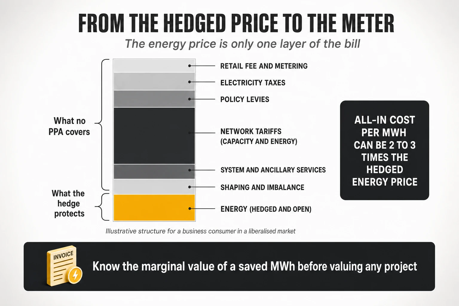
The non-energy layers are growing in several markets. Across the EU, network costs rose 8.9% in 2024 and non-recoverable taxes and levies represented 17.7% of the average non-household price in the second half of 2025 (Eurostat). In the US PJM market, the capacity auction for 2027/28 cleared at its cap of 333.44 $/MW-day, driven mainly by data-centre load (Power Engineering). As renewables grow, the system operator needs more balancing, more reserves and more constraint management, and those costs are spread over consumers’ bills independently of the energy hedge. A telco with 80% of its energy hedged can still see its unit cost rise because the parts of the bill that no hedge covers are rising.

The reconciliation that every energy team should be able to do

Consider a hypothetical operator that consumes 1,000 GWh a year through supply points it manages directly, in a European market. All figures are invented for illustration, but the structure is typical of a large business consumer. The exercise is to walk from the price of the energy contracts to the energy line in the corporate P&L in three levels, keeping track of the volume at each level.

Line	Volume	€/MWh	M€ per year	Who controls it
Hedged energy: 65% of volume at 55 €/MWh	650 GWh	55.0	35.8	Procurement
Open energy: 35% at an average market price of 80 €/MWh	350 GWh	80.0	28.0	Procurement (exposure)
Level 1 — energy bought	1,000 GWh	63.8	63.8
Shaping and imbalance		4.0	4.0	Procurement and retailer
System and ancillary services		12.0	12.0	Regulator, system operator
Network tariffs: capacity (kW) part		18.0	18.0	Regulator; operations through contracted capacity
Network tariffs: energy (kWh) part		12.0	12.0	Regulator
Policy levies		8.0	8.0	Government
Electricity tax		6.0	6.0	Government
Retail fee and metering		2.0	2.0	Procurement
Level 2 — full cost of directly managed supply	1,000 GWh	125.8	125.8
Energy re-invoiced by tower companies and landlords	80 GWh	150.0	12.0	Contracts with third parties
Offices, shops and other buildings	30 GWh	133.3	4.0	Facilities
Other items booked in the energy line (allocations, lease-accounted assets)	—	—	3.0	Finance
Level 3 — corporate energy line	1,110 GWh	about 130	144.8

Caption: An illustrative three-level reconciliation from contract prices to the corporate energy line. Hypothetical figures; components and weights vary by country and operator.

Four conclusions follow from the table.

• The “energy price” is half of the cost of supply. Even with a well-hedged portfolio, the full cost per MWh of directly managed supply (level 2) is about twice the blended energy price (level 1).
• Each level needs its own volume. The corporate line includes energy consumed outside the 1,000 GWh — on tower-company sites, in offices — so dividing 144.8 M€ by 1,000 GWh (145 €/MWh) overstates the unit cost. The correct corporate average is about 130 €/MWh over 1,110 GWh, and only level 2 is a true cost per MWh of the operator’s own supply.
• Procurement directly controls less than half of the line. Energy, shaping and retail fees add up to about 70 M€ of 145 M€. The rest is regulated, taxed, or sits in contracts that the energy team often does not manage — such as energy re-invoiced by tower companies.
• Without the walk, nobody knows what a saved MWh is worth. That is the subject of the next two subsections.

What a saved MWh avoids on the bill

The value of saving one MWh is not the average cost per MWh. In the example, a MWh not consumed avoids the energy component plus the variable parts of the bill: shaping (4 €), system charges (12 €), the energy part of network tariffs (12 €), energy-based levies (8 €) and the electricity tax (6 €) — about 42 € of variable charges. It does not avoid the capacity part of network tariffs, which depends on contracted kW, nor fixed fees. How much of the energy component it avoids depends on the contract, as the next subsection shows.

Two practical consequences follow.

• Business cases for efficiency projects should use the marginal avoided cost, state which components of the bill they avoid, and value crisis savings at the expected market price during the crisis, not at the budget’s average cost.
• Capacity charges deserve their own programme. In networks with tens of thousands of supply points, contracted capacity that no longer matches the equipment installed is a recurring and often invisible cost — 18 M€ a year in the example.

What happens to a hedge when the network consumes less

Suppose the operator switches off legacy equipment and consumes 100 GWh less per year. The market price is 80 €/MWh, the hedge price 55 €/MWh, and every MWh saved avoids about 42 € of variable charges whatever the contract. What the saving is worth on the energy component depends on how that energy was bought.

How the energy was bought	What happens when consumption falls by 100 GWh	Energy component avoided	Total avoided, including 4.2 M€ of variable charges
Indexed or spot supply	The operator simply buys 100 GWh less at the market price	8.0 M€	12.2 M€
Financial hedge (swap) with physical supply at index	Physical purchases at market fall by 100 GWh; the swap keeps settling on its fixed notional volume, unaffected	8.0 M€ (valued at spot)	12.2 M€
Fixed-price supply billed on actual consumption	The billed volume falls, within the contract’s tolerance band	5.5 M€ (at the contract price)	9.7 M€
Physical PPA with a purchase obligation, if consumption falls below the contracted volume	The operator still pays 55 €/MWh for the PPA output; the surplus is resold at the market price of the hours when it is produced (say 30 €/MWh for solar)	3.0 M€ (resale value, before fees)	7.2 M€

Caption: The value of 100 GWh of savings under four contract types. Hypothetical prices; resale and tolerance terms vary by contract.

Three points matter more than the numbers.

• A financial hedge does not destroy the value of a saving. The saving is valued at spot because the physical energy is bought at spot; the swap is a separate financial position. But if consumption falls below the swap’s notional volume, part of the hedge no longer covers anything: it becomes a bet on the price, gaining if prices rise and losing if they fall.
• Fixed-price supply passes the saving through at the contract price — as long as the reduction stays within the tolerance band. Beyond it, contracts typically apply penalties or settle the difference at market.
• Physical obligations are where savings lose most value. As long as consumption stays above the PPA volume, the saving reduces residual market purchases and is worth the spot price. Once it pushes consumption below the contracted volume, the operator keeps paying the PPA price and earns only the resale value of the surplus. This is why decommissioning plans and PPA volumes must be sized together.

7. The procurement toolbox: six ways to buy electricity

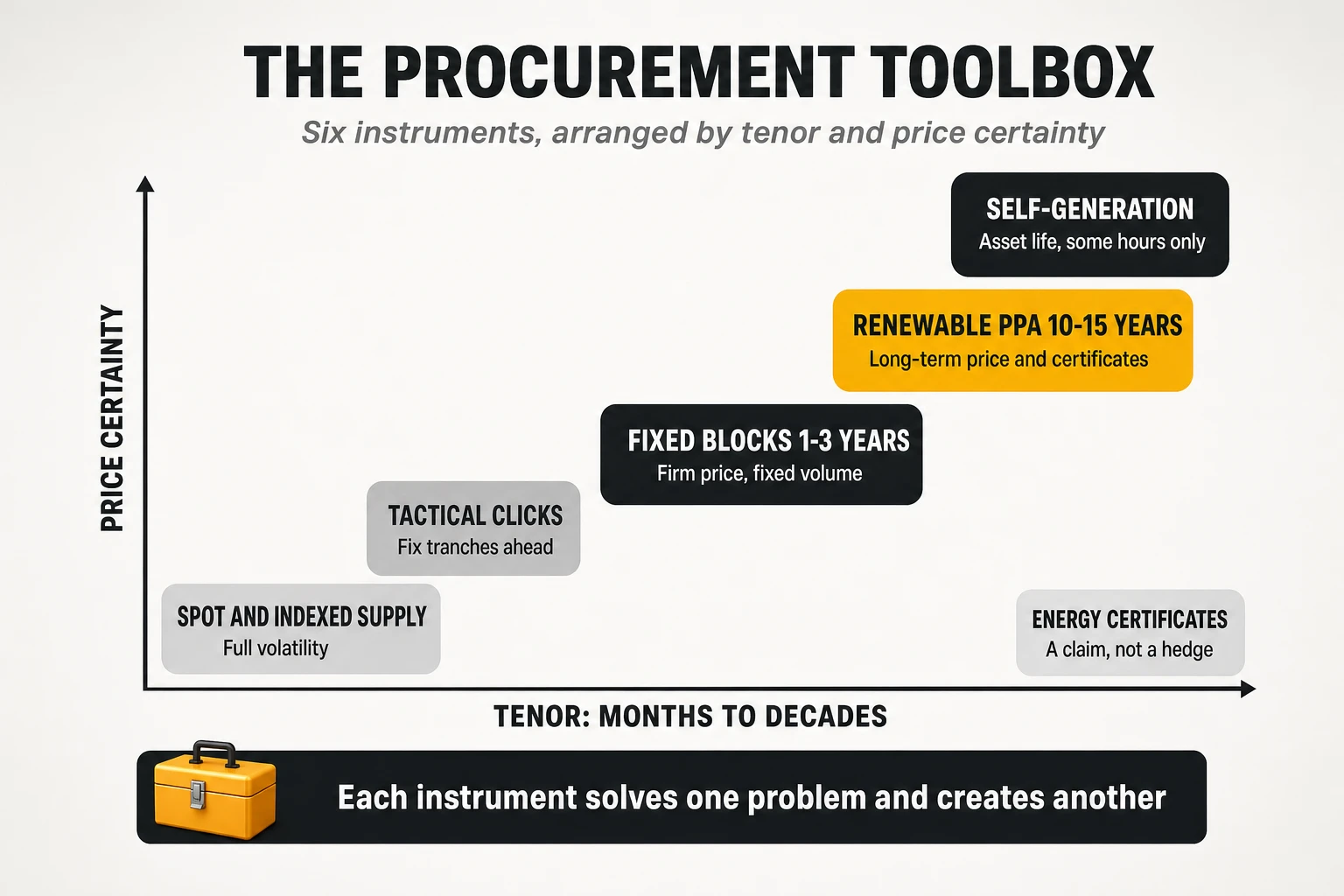
A large operator does not choose one contract for all its electricity. It builds a portfolio of instruments with different tenors, prices and risks, much as a treasury builds a debt portfolio with fixed and floating tranches. Each instrument solves one problem and creates another.

Instrument	What the telco gets	Typical tenor	Main risk it leaves behind
Renewable PPA	A fixed or structured price for the output of one or several plants, plus their certificates	10-15 years, sometimes 20	Shape and volume risk; long commitment; counterparty risk
Fixed-price supply or baseload hedge	A firm price for a defined volume and period, usually through the retailer or a forward contract	1-3 years	Over- or under-hedging if consumption changes
Tactical forward purchases (clicks)	The right to fix the price of tranches of volume progressively, months or quarters ahead	Months to 3 years	Timing; buying a tranche just before prices fall
Indexed or spot supply	Energy at the day-ahead price plus a retailer fee	Rolling	Full exposure to volatility and spikes
Self-generation	On-site or remote production that displaces grid purchases	15-25 years (asset life)	Capital or long contracts; production only in some hours
Energy attribute certificates	Renewable claim for a volume (GOs, RECs, I-RECs)	Annual	Provides a claim, not a price hedge

Caption: The six building blocks of a telco electricity portfolio. In practice several are combined in the same supply contract: for example, an indexed contract with the right to fix tranches over time.

Power purchase agreements, explained

A power purchase agreement (PPA) is a long-term contract between a buyer and a generator, usually tied to a specific renewable plant or portfolio. It fixes the price, the duration, the volume and its profile, who absorbs which risks, and who keeps the environmental attributes (the guarantees of origin or renewable energy certificates). Corporate PPAs became the main instrument for large buyers in the 2010s because they lock a price for a decade and let the buyer claim additional renewable capacity. Corporations signed 55.9 GW of clean-energy PPAs worldwide in 2025, the second-highest year on record after 62.2 GW in 2024, with the four largest technology companies accounting for 49% of the total (BloombergNEF via pv magazine).

Three structures cover most of the market.

• Physical PPA. The energy is contractually delivered to the buyer, normally through a retailer that “sleeves” it — integrates the plant’s output into the buyer’s supply contract, schedules it and supplies the difference between what the plant produces and what the buyer consumes. The network is still the shared grid; the delivery is commercial. Section 9 follows one such contract through a month, step by step.
• Virtual or financial PPA (VPPA). The buyer keeps buying electricity from its usual supplier at market prices. Separately, it settles the difference with the generator: if the market reference is below the agreed fixed price (the “strike price”), the buyer pays the difference; if it is above, the generator pays the buyer. Economically it is a long-term swap, a contract for difference. Its effectiveness depends on how closely the market reference used for settlement matches the price the buyer pays for its own consumption.
• Baseload or structured PPA. The seller commits to deliver a defined shape — for example, a constant megawatt every hour — and uses its own portfolio, storage and market purchases to fill the gaps of the renewable plant. It suits a 24/7 consumer far better, but the seller charges for the risk it takes.

Inside each structure, the volume definition decides who carries the weather risk: under pay-as-produced the buyer takes whatever the plant generates (usually the lowest price, the most risk for the buyer); under pay-as-forecast it takes a pre-agreed profile; under a baseload or shaped definition it receives a fixed profile and the seller charges a premium for absorbing deviations.

Shape risk: why a cheap solar PPA is not cheap electricity for a network

Consider a site that consumes 10 kWh every hour of the day, 240 kWh in total. The operator signs a solar PPA sized to produce 240 kWh per day on average. On paper the site is 100% covered. Hour by hour it is not.

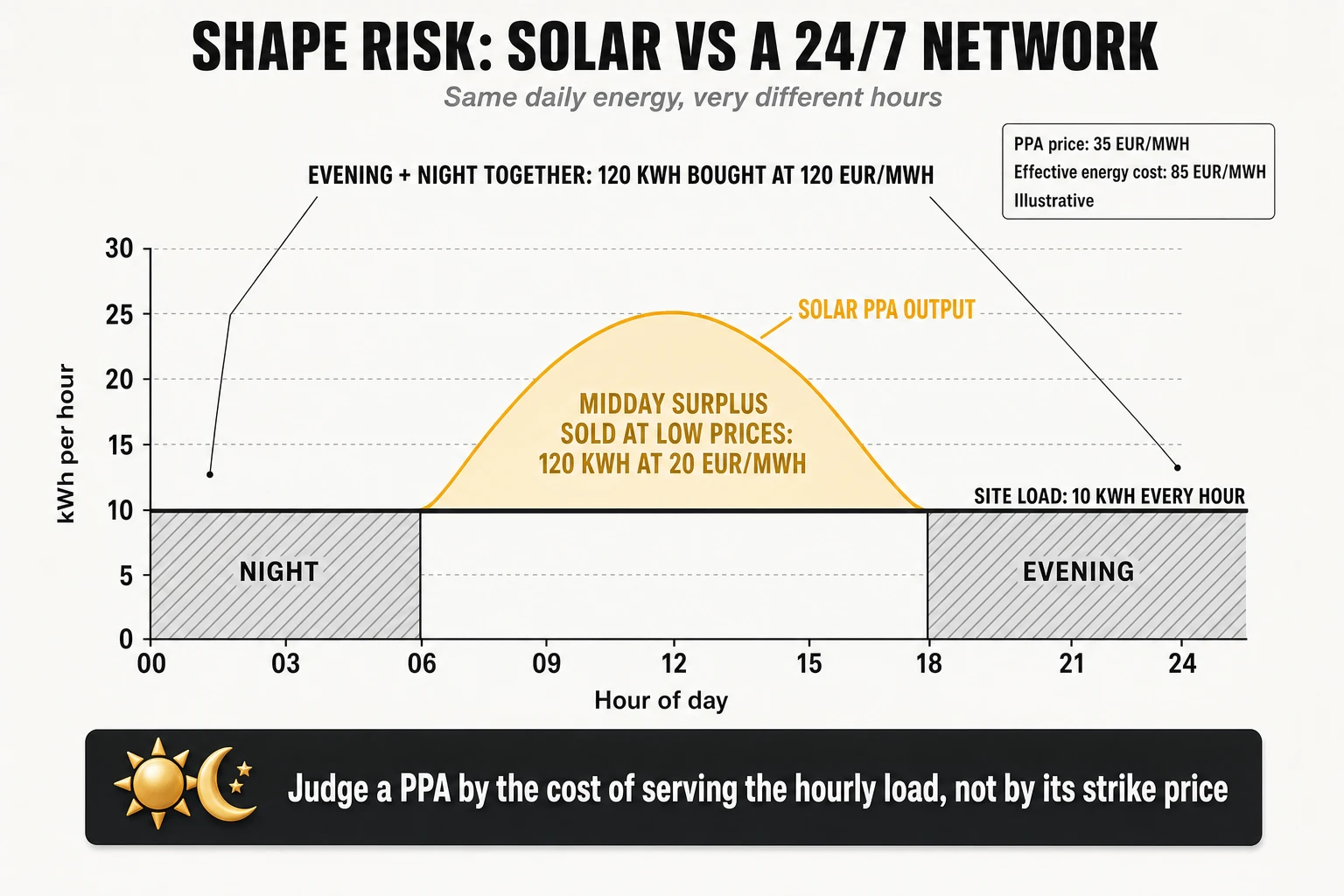
Around midday, the plant produces more than the site consumes, and the surplus is sold back when solar has pushed prices down, sometimes below zero — Germany recorded 576 negative-price hours in 2025, up from 440 in 2024 (Electricity Maps). From sunset to sunrise it produces nothing, and the site buys its energy in the evening and night hours, usually the most expensive of the day. This is shape or profile risk, the most underestimated element of corporate PPAs: the relevant metric is the total cost of serving the hourly load, not the strike price.

The same example, in euros

Put prices on the same site. Suppose that half of the solar output (120 kWh) coincides with the site’s consumption, the other half (120 kWh) is surplus sold back at midday, and the site buys 120 kWh in the evening and at night. The prices are illustrative but realistic for a market with a lot of solar.

Item	Energy	Price	Cost per day
Solar PPA: all output paid at the strike price	240 kWh	35 €/MWh	8.40 €
Evening and night energy bought from the market	120 kWh	120 €/MWh	+ 14.40 €
Midday surplus sold back to the market	120 kWh	20 €/MWh	− 2.40 €
Net cost of the 240 kWh consumed	240 kWh	85 €/MWh	20.40 €

Caption: Effective energy cost of a 35 €/MWh solar PPA serving a flat load. Illustrative prices; excludes network tariffs, system charges and taxes.

The headline price is 35 €/MWh; the effective energy cost is 85 €/MWh — almost two and a half times more. The difference has nothing to do with the quality of the negotiation. It comes from the shape of the load, the shape of the plant’s output and the spread between solar hours and night hours. If that spread widens — more solar in the system, a gas shock in the evening hours — the effective cost rises even though the PPA price has not moved.

How PPA prices differ by product

Market references make the trade-off visible. In the second quarter of 2026, LevelTen Energy’s index put the P25 offer price of European solar PPAs at about 56.6 €/MWh and of European wind PPAs at about 96 $/MWh, with its new hybrid (renewables plus storage) index priced roughly 24% above solar and 15% below wind; in North America, solar stood at 61.40 $/MWh and wind at 83.79 $/MWh (LevelTen via PV Tech). Pexapark’s European composite stood at 48.34 €/MWh in September 2026 (PV Tech). These are offer and index references, not the cost of serving a load.

The general pattern holds in many markets, with exceptions: in sunny markets, pay-as-produced solar tends to be the lowest-priced product; wind is often priced higher because its profile is more valuable, although in windy markets it can be cheaper than solar; and baseload or shaped products are usually the most expensive, because the seller is pricing the risk of filling the hours when the plants do not produce. Location, tenor, start date, contract structure and the actual production profile of each site change the ranking. A buyer comparing headline prices across these products is comparing different goods, which is why section 8 compares them on the cost of serving the load.

What is changing in PPA contracts

Solar cannibalisation and negative prices have pushed buyers and sellers to redesign contracts. The main changes are clauses that suspend payment when the market price is below zero; floors and caps (a “collar”) instead of a single fixed price; hybrid PPAs in which a battery shifts solar output into the evening; portfolio PPAs that combine solar and wind from several sites; multi-buyer deals for mid-sized buyers; and, in Europe, public guarantee schemes and two-sided contracts for difference promoted by the 2024 market reform (Regulation (EU) 2024/1747).

Accounting is part of the decision

A PPA can look very different in the financial statements depending on its structure. A physical PPA for own use is normally treated as an executory supply contract. A virtual PPA is a derivative under IFRS 9 and US GAAP (ASC 815): unless it qualifies for hedge accounting, its mark-to-market value — what the contract would be worth if closed at today’s prices — goes through the income statement every quarter, creating volatility that has nothing to do with operations. The IASB amended IFRS 9 in December 2024, effective from January 2026, to ease the own-use assessment and allow hedge accounting for contracts referencing nature-dependent electricity such as solar and wind PPAs (EY summary); in the US, virtual PPAs generally fail the normal-purchases exception of ASC 815 and are treated as derivatives (PwC Viewpoint). Treasury and accounting must be involved before the term sheet, not after.

8. Building the hedge portfolio

Hedging is not about buying at the bottom of the market. It is about making the energy cost of the next years predictable enough for the budget, at a price that is competitive on average, within a level of risk that the board has explicitly accepted. The operator that tries to time the market with its whole volume is speculating with the P&L, whether it calls it that or not.

How a hedge works: a simple example

Suppose an operator expects to consume 100 GWh in 2028 and today fixes 60 GWh at 55 €/MWh. When 2028 arrives:

• The 60 GWh hedged cost 55 €/MWh, whatever the market does (as long as the contract’s profile and volume conditions are met).
• The remaining 40 GWh are bought at the prices of 2028.
• If the market averages 100 €/MWh, the hedge saved 2.7 M€ against buying everything at spot.
• If the market averages 40 €/MWh, the hedge cost 0.9 M€ more than buying everything at spot.

Both outcomes are acceptable if the hedge was a decision about risk, not a bet on price. A hedge that “lost money” in a falling market did its job: it removed the possibility of a much larger loss in a rising one. Reporting hedges as gains or losses against spot, without that context, is how hedging programmes get cancelled at exactly the wrong moment.

Core, tactical and open: a three-layer architecture

A useful way to organise the portfolio is in three layers with different tenors and purposes. The weights are a decision of each company, not an industry standard; the ranges below are illustrative.

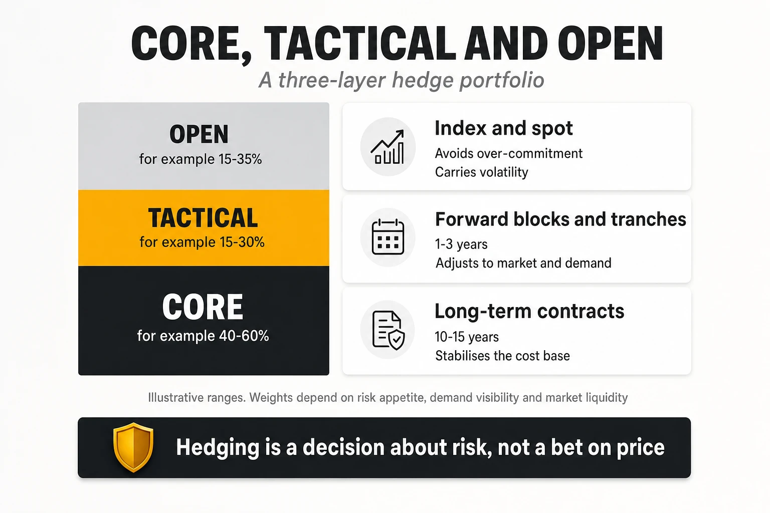
The core layer (for example 40-60% of expected consumption) holds long-term PPAs and structural contracts that stabilise the cost base for 10-15 years. The tactical layer (for example 15-30%) holds forward blocks for the next one to three years, bought in tranches to adjust to the market and to consumption. The open position (for example 15-35%) is bought at index or spot, avoiding over-commitment if consumption or prices fall.

The right weights depend on four things: the budget volatility the company can tolerate; how predictable consumption is over the horizon (a network in the middle of a large decommissioning programme should not commit 60% of today’s volume for fifteen years); the liquidity of local forward and PPA markets; and the contracts already held.

Which portfolio? Four strategies compared

Describing instruments is not enough; the operator has to choose a combination. To show how that choice can be made, take a hypothetical operator with a load of 1,000 GWh a year and compare four portfolios in a single delivery year, with all contracts already in place, using a simple, transparent model.

The assumptions are deliberately simple and fully illustrative:

• The load is simplified as flat: 400 GWh fall in “solar hours” (when solar plants produce) and 600 GWh in the rest of the day and night.
• Three market scenarios for that year, with different prices in solar hours and in the rest. Low (renewable surplus, cheap gas): 10 and 70 €/MWh. Base: 30 and 95 €/MWh. Crisis (gas shock): 70 and 210 €/MWh. The market-only average for a flat load is therefore 46, 69 and 154 €/MWh.
• Contract prices: solar PPA at 35 €/MWh, producing only in solar hours; wind PPA at 50 €/MWh, producing 40% in solar hours and 60% in the rest; baseload supply at 68 €/MWh; forward blocks bought in tranches at an average of 72 €/MWh. All contract volumes are paid; surpluses are sold back at the market price of the hour; shortfalls are bought at market.
• Only the energy component is modelled; network tariffs, system charges and taxes are the same in all strategies.

Strategy	Contracts	Net market purchases in non-solar hours	Low	Base	Crisis	Crisis minus base
Market only	None	600 GWh	46.0	69.0	154.0	85.0
A. Solar-heavy	70% solar PPA, rest at market	600 GWh (plus 300 GWh of midday surplus resold)	63.5	72.5	129.5	57.0
B. Solar and wind	35% solar PPA, 35% wind PPA, rest at market	390 GWh	56.2	64.1	105.4	41.3
C. Baseload	70% baseload supply, rest at market	180 GWh	61.4	68.3	93.8	25.5
D. Diversified	20% solar, 20% wind, 40% forward blocks, 20% market	240 GWh	62.2	67.4	93.4	26.0

Caption: Energy cost in €/MWh (equal to M€ for 1,000 GWh) in one delivery year under three market scenarios. Hypothetical operator and prices; the results hold only under these assumptions and show the method, not a recommendation.

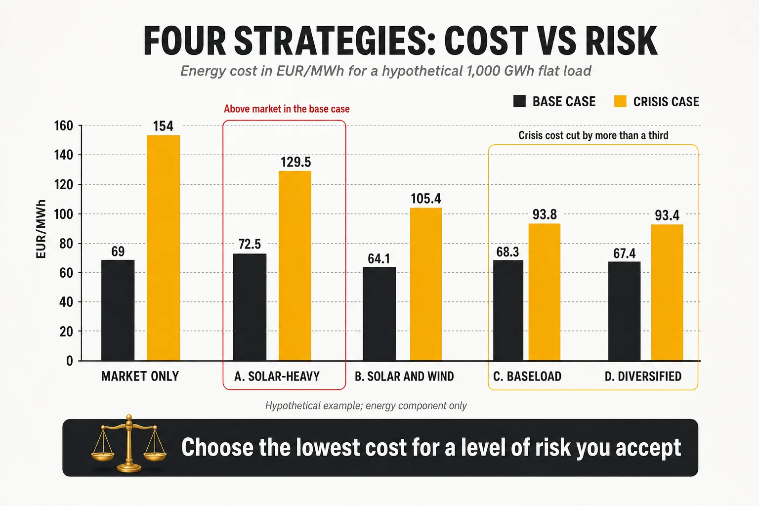
Read the results as a comparison for one delivery year, under these assumptions only. Five observations follow.

• The solar-heavy portfolio is the least favourable here. Being “70% covered” by a 35 €/MWh PPA costs 72.5 €/MWh in the base case — more than buying everything at market — because 300 GWh of midday surplus are resold at 30 €/MWh while all 600 GWh of night-time energy are still bought at market. In a crisis it absorbs less than a third of the price increase.
• Diversifying technologies lowers the base-case cost. Combining solar and wind (B) gives the lowest base-case and expected cost, because the wind contract delivers part of its energy in the expensive hours. But it leaves 390 GWh exposed at night and costs 105.4 €/MWh in a crisis.
• Flat products buy protection. Baseload supply (C) and the mix with forward blocks (D) cost about 94 €/MWh in a crisis: about 60 €/MWh, or almost 40%, less than buying everything at market.
• Compared with B, that protection has a price. With weights of 25% low, 60% base and 15% crisis, the expected costs are 76.0 (market only), 78.8 (A), 68.3 (B), 70.4 (C) and 70.0 (D) €/MWh. Moving from B to C costs about 2.1 €/MWh of expected cost and saves about 11.6 €/MWh in the crisis year; moving from B to D costs about 1.7 €/MWh and saves about 12.0 €/MWh. That is the kind of trade-off a board can understand and decide.
• Flexibility has a value the table does not show. Strategy D commits only 40% of volume to long-term contracts; its forward blocks can be resized as decommissioning reduces consumption.

A ten-year decision needs a ten-year model. The PPAs and baseload contracts in the example last ten years, while forward blocks are usually bought one to three years ahead and must be renewed at whatever prices prevail. In a crisis lasting several years, the blocks of strategy D would be renewed at crisis prices and its advantage over B would shrink; in a long period of low prices, every hedged strategy would look expensive. A real strategic comparison would add renewal prices for the short instruments, several weather years and hourly price profiles, the expected evolution of consumption, and a probability distribution of scenarios. No combination of solar, wind, baseload and market wins in every country and every scenario. The question such a model must answer stays the same: which portfolio gives the lowest cost for a level of risk the company is willing to accept, for a network that consumes 24 hours a day?

Layered purchasing and hedge ratios by horizon

The tactical layer is normally executed as a staircase. The operator defines a minimum hedge ratio for each future year that rises as delivery approaches, and buys in regular tranches to reach it.

Delivery year	Minimum hedged share	Maximum hedged share	How it is reached
Next year (Y+1)	70-80%	90-95%	Quarterly tranches during the current year
Y+2	50-60%	75%	Semi-annual tranches
Y+3	30-40%	60%	Opportunistic tranches below a target price, plus PPAs
Y+4 and beyond	Core layer only	50%	Long-term contracts

Caption: An example of a hedge-ratio policy by horizon. The numbers are illustrative; each company sets them according to its risk appetite, demand visibility and market liquidity.

Two kinds of triggers move purchases forward or back. Time triggers ensure that the minimum ratio is reached by a given date regardless of price; price triggers allow faster buying when the forward curve falls below a target, or slower buying when it spikes. The combination avoids both paralysis and panic buying.

The hedge cliff

The most important chart in a telco energy review is the hedged share by year over the next ten years. Long-term PPAs signed before the 2021-2022 crisis expire on fixed dates; as they do, the protected share falls in steps, and the cost of replacing it is set by the market at renewal, not by the expiring contract.

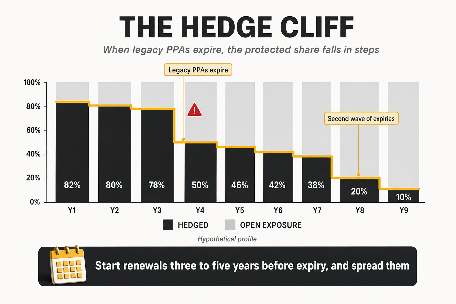
For the hypothetical 1,000 GWh operator, the sensitivities are easy to compute. With 80% hedged, a 50 €/MWh rise on the 200 GWh open adds 10 M€ a year; if the hedged share falls to 50%, the same rise on 500 GWh adds 25 M€. If the expiring contracts were 30 €/MWh below today’s replacement cost on 300 GWh, renewal alone adds another 9 M€ a year. These are sensitivities, not forecasts — and they show why renewals deserve as much attention as the network investment plan. The two worst approaches are symmetrical: renewing everything in the last year at whatever the market offers, or locking ten years of volume in one week because gas has just spiked.

Risk metrics and counterparty risk

Hedging policies survive when they are expressed in the language of the CFO. Three metrics do it: budget at risk, the cost overrun that would occur in, say, the worst 5% of price scenarios over the next 12-24 months; cost per MWh by scenario, with hedged and open parts shown separately, as in the strategy comparison; and sensitivity, the millions the bill moves per €/MWh of market change (0.2 M€ with 200 GWh open, 0.5 M€ with 500 GWh). They make the hedge cliff visible years before it arrives.

A long-term contract is only as good as the company on the other side. A generator that defaults during a price spike removes the hedge exactly when it is most valuable; conversely, lenders financing the plant will scrutinise the buyer’s credit. Credit support, diversification across counterparties and termination clauses with replacement-cost compensation matter as much as the strike price.

9. How electricity contracts work and are negotiated

Negotiating a PPA or a large supply contract is closer to negotiating a project finance deal than to buying a commodity. The price matters, but the clauses that allocate risk — volume, shape, curtailment, negative prices, change in law, credit, termination — often matter more over a ten-year life. An operator that negotiates only the headline €/MWh usually discovers the rest of the contract when something goes wrong.

How a physical PPA actually runs: one month, step by step

Before looking at negotiation, it helps to follow a contract through one month of operation. Take a hypothetical operator that consumes 8 GWh a month and has a ten-year physical PPA with a wind and solar portfolio, pay-as-produced, at 50 €/MWh. A retailer “sleeves” the PPA: it integrates the plant’s output into the operator’s supply and provides everything else.

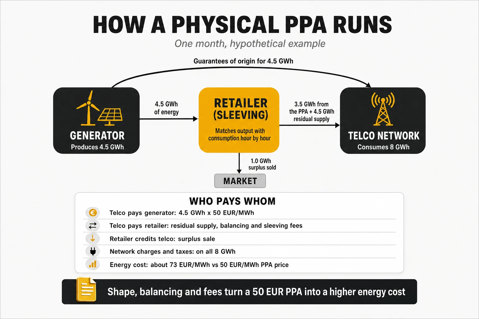
1. The plant produces 4.5 GWh, less than the 5 GWh expected, because the month was calm. Under pay-as-produced, the operator pays the generator for exactly what was produced: 4.5 GWh × 50 €/MWh = 225,000 €. Nobody compensates the missing 0.5 GWh.
2. The retailer matches production and consumption hour by hour. In this month, 3.5 GWh of the plant’s output fall in hours when the network is consuming it; 1.0 GWh falls in hours when the plant produces more than the network uses (sunny, windy middays).
3. The surplus is sold. The retailer sells the 1.0 GWh in the market at the price of those hours, say 25 €/MWh, and credits 25,000 € to the operator.
4. The rest of the consumption is supplied by the retailer. The network needs 8 GWh; the PPA covered 3.5 GWh in the right hours, so the retailer supplies 4.5 GWh at the market or contract price, say 80 €/MWh: 360,000 €.
5. Deviations are settled. The plant’s actual output differs hour by hour from its forecast; the resulting imbalance cost is charged by the system operator to whoever is responsible for balancing — here the retailer, which passes it on as a fee, say 2 €/MWh on the PPA volume: 9,000 €.
6. The retailer charges for its service — sleeving and shaping, say 3 €/MWh on the PPA volume: 13,500 €.
7. Regulated charges are billed on total consumption. Network tariffs, system charges, levies and taxes apply to all 8 GWh, exactly as they would without a PPA.
8. The certificates move. The generator transfers guarantees of origin for 4.5 GWh to the operator through the national registry; they support its renewable claim.

The energy cost of the month is 225,000 + 360,000 − 25,000 + 9,000 + 13,500 = 582,500 €, or about 72.8 €/MWh for 8 GWh — before regulated charges. The PPA price was 50 €/MWh. The difference comes from the hours the plant did not cover, the surplus sold below cost and the fees, which is why shape and balancing terms matter as much as the price.

Two variations change the picture.

• If the contract were baseload or pay-as-forecast, the generator would have to deliver the agreed profile or compensate the shortfall — usually at the market cost of replacing it — and would charge a higher price for taking that risk.
• If it were a virtual PPA, the operator would buy all 8 GWh from its retailer at market prices and, separately, settle with the generator on the 4.5 GWh produced: if the market reference averaged 60 €/MWh, the generator would pay the operator (60 − 50) × 4,500 MWh = 45,000 €; if it averaged 40 €/MWh, the operator would pay 45,000 €. No energy changes hands; certificates are transferred separately.

Contract terms in plain words

Term	What it means
Strike price	The fixed price agreed in a PPA or swap
Sleeving	A retailer integrating a PPA into the buyer’s supply and handling everything around it
Pay-as-produced / pay-as-forecast / baseload	Whether the buyer takes actual output, a forecast profile or a fixed hourly profile
Imbalance	The difference between scheduled and actual production or consumption, charged by the system operator
Curtailment	An order from the grid operator to reduce a plant’s output, usually because of congestion
Settlement point	The market price (zone, hub or node) used to calculate payments in a virtual PPA
Collar	A price range with a floor and a cap, instead of a single fixed price
Take-or-pay	An obligation to pay for a contracted volume whether or not it is used
Mark-to-market	The value of a contract if it were closed at today’s market prices
Credit support	Collateral or guarantees each party posts to protect the other against default
Change in law	A clause on who bears the cost of new taxes or market rules

Caption: The vocabulary of electricity contracts, explained.

What a telco brings to the table

Telecom operators are attractive offtakers and should negotiate as such: a large, round-the-clock load that few buyers can match for ten years; investment-grade credit in most cases, which makes a PPA bankable; thousands of supply points that give retailers scale; and a sustainability story that generators value. Their weaknesses are just as real: consumption falls in legacy segments and rises in others, the load is spread over small low-voltage sites, and operators that sold their towers buy part of their energy through third parties.

The process, step by step

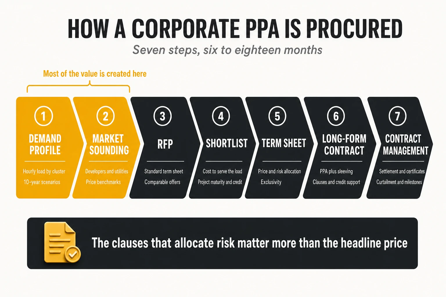
1. Demand profile and strategy: hourly consumption by site cluster, projected with decommissioning and growth; what the portfolio needs in volume, technology mix, shape, tenor and accounting treatment.
2. Market sounding: developers, utilities and advisers test appetite; prices are benchmarked against published PPA indices.
3. Request for proposals: a standard term sheet so that offers are comparable.
4. Shortlist: offers compared on the cost of serving the load, risk, counterparty strength and project maturity (permits, grid connection, financing).
5. Term sheet: economic and risk terms agreed with one or two bidders.
6. Long-form contract: usually based on market templates (EFET in Europe, EEI-based forms in the US), plus the sleeving agreement.
7. Contract management: production, settlement, certificates, curtailment and project milestones.

The process typically takes six to eighteen months. Operators that start it when a hedge expires negotiate under time pressure, the weakest position in any negotiation.

The clauses that decide the real price

Clause	The question it answers	What a telco should seek
Price structure	Fixed, indexed, escalating, collar?	Fixed or collar with moderate escalation; avoid uncapped indexation
Volume definition	Pay-as-produced, as-forecast, baseload?	As close to the load shape as the budget allows; volume bands of ±10-20%
Settlement point (virtual PPA)	Which market price is used to settle?	A hub or zone that tracks the operator’s own purchase price
Negative prices	Who pays when the market is below zero?	No payment obligation in negative hours
Curtailment	What if the grid operator limits production?	Compensation or volume make-up, not silent loss of hedge
Commercial operation date	What if the plant is late?	Delay damages and a long-stop date with exit rights
Change in law	Who bears new taxes or market rules?	Balanced sharing, with renegotiation triggers
Certificates	Who gets the guarantees of origin, and how?	Transferred monthly, matched to the volume
Credit support	What collateral does each side post?	Symmetrical, rating-based, with caps
Termination and assignment	What if one side exits, defaults or sells assets?	Mark-to-market termination payment; the right to transfer the contract if towers, data centres or networks are sold
Volume flexibility	What if consumption falls?	Right to reduce volume or resell surplus at predefined terms

Caption: The clauses that determine the effective cost and risk of a corporate PPA. Headline price comparisons that ignore them are misleading.

Negotiating with the retailer

For most telcos, the retailer contract matters as much as the PPAs, because the retailer supplies the residual volume, sleeves the PPAs, absorbs imbalances, manages tens of thousands of metering points and sends the invoices. The points to negotiate are capped and benchmarked fees for sleeving, shaping and balancing; clear pass-through rules for system charges; the right to fix tranches of indexed volume at forward prices (“clicks”) with transparent spreads; hourly consumption data per supply point in a usable format; and invoice-validation rules, because across thousands of points billing errors are worth more than many efficiency projects.

The three most expensive mistakes are buying the cheapest MWh instead of the cheapest load served, sizing ten-year volumes without a demand plan, and concentrating renewals in the same year — which guarantees that the cliff repeats every cycle.

10. The other half of the equation: managing demand

Every MWh that the network does not consume is a MWh that does not have to be bought, hedged, shaped, transported or taxed. Demand reduction is the only lever that improves price exposure, cost level and emissions at the same time. It is also the lever that is most often managed separately from procurement, by different teams, with different numbers.

Where the savings come from

Telco efficiency programmes fall into five families, with very different economics.

• Decommissioning legacy networks. Switching off copper exchanges, PSTN switches, 2G/3G layers, old transport platforms and IP equipment that carries little traffic. These projects deliver the largest savings, but they depend on customer migration, regulatory approval and site sales. Analysys Mason estimates that switching off 2G/3G can cut macro-site energy by up to 40% and that a full FTTP network can cut access energy by up to 80% compared with copper; BT has measured FTTP at about 13% of the energy per line of FTTC, and Telenor expects copper switch-off to save up to 100 GWh a year, about one-eighth of its total (Analysys Mason). Across 14 operators in advanced markets, the GSMA found that electricity consumption fell 4.5% a year after the 3G sunset, against 2% a year in the two years before (GSMA Mobile Net Zero 2026).
• Modernising active equipment. Replacing old radio units, OLTs and routers with newer generations that deliver more capacity per watt. The saving is usually a by-product of a capacity or obsolescence investment.
• Radio energy features. Carrier, channel and symbol shutdown in low-traffic periods, deep sleep for power amplifiers, AI-driven scheduling of those features by cell. Measured results are smaller than vendor claims but material: a Vodafone UK trial with Ericsson reduced the daily power use of 5G radio units at selected London sites by up to 33% (TelecomTV), and an MTN South Africa trial with ZTE raised per-site savings from 2.8% to 13.5% with AI-driven control (Developing Telecoms). McKinsey puts the typical gain from AI tools at 5-7% (McKinsey).
• Cooling and building systems. Free cooling, higher temperature set points in equipment rooms, replacement of old air-conditioning units, containment in data centres.
• Data centre consolidation. Closing small, inefficient server rooms and moving workloads to fewer, better facilities with lower PUE (power usage effectiveness: total facility energy divided by IT energy).

Measuring savings honestly

An efficiency programme is only as credible as its measurement. Many report savings as the difference between a projected baseline and the actual consumption, without controlling for weather, traffic, new sites or migrations. Three practices separate credible programmes from optimistic ones:

• A plan, a trajectory and an outturn. Track the original target, the current committed trajectory and the realised savings separately, by initiative. A programme that meets its total only because one initiative over-delivers while others slip is less robust than its headline suggests.
• Measurement and verification at site level where possible, using metered data before and after, or regression models adjusted for temperature and traffic. These are also the methods that public efficiency incentive schemes require to award support.
• Equipment counts as a leading indicator. The number of devices actually switched off versus the number planned is often the earliest signal that a programme is slipping.

Demand levers in a price crisis

When prices spike, the demand side is the only lever that acts immediately on the open volume. Hedges cannot be bought retroactively, but consumption can be changed in a matter of weeks. Three different effects should not be confused:

• Energy saving reduces the MWh consumed — switching off equipment, raising set points. It lowers the bill permanently or for the duration of the measure.
• Load shifting moves consumption from expensive to cheaper hours — running sites on batteries at the evening peak and recharging later. Total energy is similar (slightly higher, because of battery losses); the saving comes from the price spread.
• Peak reduction lowers the maximum power drawn at a site. It reduces capacity charges and contracted power, not energy.

The levers below combine these effects and differ in speed and in the risk they carry for service.

Lever	What it involves	Speed	Main constraint
Peak shaving with site batteries	Running selected sites on their batteries during peak hours, within the autonomy reserved for outages	Days	Battery condition and minimum backup autonomy
Load reduction on request	Joining national demand-reduction schemes at peak hours	Weeks	Must not affect emergency services or critical traffic
Accelerating planned switch-offs	Bringing forward decommissioning of legacy platforms and sites already scheduled	Months	Customer migration and regulatory approvals
Cooling set points and maintenance	Raising equipment-room temperatures within manufacturer specifications; fixing faulty units	Weeks	Equipment warranties and failure rates
Radio energy features	Extending low-traffic shutdown windows and activating features already licensed	Weeks	Coverage and quality commitments
Idle equipment	Switching off unused cards, ports and nodes	Weeks	Inventory accuracy

Caption: Demand levers for a price crisis, from fastest to slowest. Each action should be valued at the expected market price of the open volume during the crisis.

Public examples show what is feasible at scale. In the winter of 2022-2023, Orange committed in France to reduce its instantaneous consumption by 5-10% for one hour a day during grid alerts, and planned to switch several thousand fixed sites to batteries at peak times, for up to 20 MW of load reduction (Light Reading). KPN, facing 50-60 million euros of additional energy cost, accelerated a savings programme on top of a 45% reduction in absolute energy use since 2010 (KPN).

The lesson is preparation. Crisis levers work only if they were identified, tested and approved before the crisis: which sites can run on batteries and for how long, which set points are safe, which switch-offs can be brought forward. An operator that starts that analysis when prices have already tripled loses the first, most expensive quarter.

Demand and procurement must share one plan

Decommissioning changes the volume that procurement has to buy, and procurement contracts constrain the value that decommissioning creates. If an operator signs ten-year PPAs sized on today’s consumption while its network plan cuts 20% of that consumption over the same period, it will end up over-hedged, reselling surplus energy at market prices that may be lower than its contracts. If decommissioning is delayed, the opposite happens: consumption exceeds the hedge and the excess is bought at spot.

The fix is organisational, not technical. One demand scenario, owned jointly by the network and energy teams, updated quarterly, with three variants — plan, delay and acceleration — and used for both the network roadmap and the hedge policy. The PPA volume bands and resale rights negotiated in section 9 are the contractual counterpart of that scenario.

11. Monetising savings and flexibility

A saved MWh lowers the bill. In many countries it can also earn money from a third party. Governments that have committed to energy-efficiency targets encourage efficiency investments in two broad ways: by paying or relieving part of the cost themselves, or by obliging energy companies to deliver savings and letting them buy savings achieved by others. In both cases, the company that invested is rewarded only for savings it can prove. For a telco running large decommissioning and modernisation programmes, part of that work can qualify.

Two different mechanisms: public support and certified savings

Mechanism	Who pays the telco	How it works	Typical conditions
Direct grants for efficiency investments	A public programme	A share of the investment is paid, often co-funded by national or regional funds	Application before investing; eligible technologies; savings verified after completion
Tax incentives	The state, through lower taxes	Tax credits, deductions or accelerated depreciation for efficient equipment	Equipment on an eligible list; documentation for the tax authority
Subsidised financing	A public lender or guarantor	Low-interest loans or guarantees for efficiency projects	Technical due diligence; repayment from the savings
Savings auctions	The authority	The authority buys a volume of savings at a competitive price	Bidding, delivery commitments, penalties for shortfall
Certified savings schemes (often called white certificates)	An energy company with a savings obligation, or an authorised intermediary	The telco transfers the rights to its verified savings under a bilateral agreement, in exchange for an agreed price	Standard methods or measured baselines; accredited verification; certificates issued by the authority

Caption: The main mechanisms that reward energy efficiency. In the first four the state pays; in certified savings schemes the state sets the rules and certifies, but the buyer is an obligated company. Names, values and rules vary by country.

The distinction matters. In a certified savings scheme, the authority does not buy the savings: it obliges energy suppliers to deliver a quantity of savings every year, and they meet part of that obligation by acquiring savings achieved by others. The telco’s counterparty is therefore a company, the price is negotiated, and the terms — when the price is paid, who carries the risk of a failed verification — are written in a contract.

The common thread is proof. Whatever the mechanism, the money depends on demonstrating to a public body, or to an accredited verifier acting for it, that a specific investment produced a specific, measurable reduction in energy use that would not have happened otherwise. Savings that do not survive the audit are not paid.

A certified savings project, from start to finish

Consider a telco that switches off a legacy platform and replaces old cooling units in 40 buildings.

1. Prepare. It identifies the eligible actions, documents the baseline consumption and agrees the measurement method, usually before the work starts.
2. Invest. It executes the project and keeps the evidence: inventories, invoices, commissioning records, metered consumption before and after.
3. Negotiate the transfer. It agrees with an obligated energy company or an authorised intermediary to transfer the rights to the savings, at a price per MWh saved. The contract defines whether payment comes at signature, at verification, at issuance or in stages.
4. Verify. An accredited verifier checks the evidence and the calculation; unproven savings are cut.
5. Issue. The authority issues the certificates — often to the buyer that requested them, not to the telco.
6. Get paid. The telco receives the agreed consideration according to the contract; authorities may audit the projects years later.

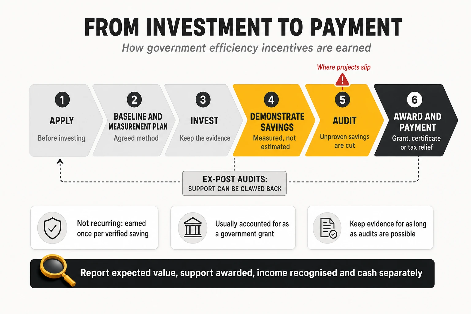
Four numbers must be tracked separately. The contracted value (what transfer agreements and grant awards promise), the certificates or grants issued, the income recognised in the accounts and the cash received. They arrive at different moments and in a different order depending on the contract: cash can come before or after issuance, and accounting recognition can precede cash.

The accounting treatment must be agreed with the auditors before the programme is reported. Public grants are normally accounted for as government grants — under IFRS (IAS 20), recognised once there is reasonable assurance that the conditions will be met and the money received, and, when they relate to an investment, spread over the life of the asset. Consideration received for transferring certified savings comes from a company under a contract; some accounting frameworks treat it by analogy with an investment grant, others as other income. In either case, recognition may occur before the cash arrives.

Three further cautions apply.

• This income is not recurring. It is earned once per verified saving (or per period of the eligible life), and a programme that reports it as a run-rate will disappoint.
• Measurement methods can fail. Baselines must be statistically robust; sites that changed use, equipment or traffic during the baseline period can invalidate a whole batch of projects. Methods should be agreed with the verifier before the project starts.
• Audits do not end with payment. Keep the evidence for as long as the authority can audit, and make sure decommissioned equipment is not reinstated in ways that cancel the saving.

The economics can be significant. Where the value per MWh saved is comparable to the price of energy, a project that saves 10 GWh a year can generate several hundred thousand euros of lower bills every year plus a one-off payment for the savings over its eligible life. For large decommissioning programmes, this can reach tens of millions of euros and change the business case for switching off legacy networks early.

Flexibility: getting paid for being able to change consumption

Many mobile sites and exchanges have backup batteries, and data centres have UPS systems. Part of that storage can, within limits, reduce consumption at peak hours or provide services that the grid operator pays for — frequency reserves, demand response, capacity — and arbitrage between cheap and expensive hours. The limits are real: battery capacity and condition vary widely, cycling shortens battery life, maintenance costs rise, and a minimum autonomy must always be kept for outages. The usable share has to be established site by site before any revenue is promised.

The best-documented telco case is Elisa in Finland, whose pooled base-station batteries were pre-qualified by the grid operator Fingrid for automatic frequency restoration reserve after a trial on 200 sites (Elisa); in 2023 the company described revenue of 30,000-60,000 euros a month and a payback of about five years (The Mobile Network), without audited figures. Technical limits apply: research by Aalto University with Telia found that site rectifiers react in 5-8 seconds, too slow for the fastest reserves (Aalto University).

The revenue is volatile and can saturate quickly as more batteries enter the market — Modo Energy reports the first signs of saturation in German reserve prices in 2026 (Modo Energy). Flexibility is a useful revenue line, not an energy strategy.

12. What operators are doing: procurement and self-production around the world

Public disclosures show the toolbox in use, with very different mixes by region. The best sector benchmark comes from the GSMA: the 18 operators that are members of RE100 bought 32 TWh of renewable electricity in 2024, of which 33% came through PPAs, 45% from unbundled certificates and 22% from green tariffs and other instruments (GSMA Mobile Net Zero 2026). In other words, even among the most committed operators, most of the renewable claim still rests on certificates, not on long-term price protection.

Long-term contracts: selected operator cases

Operator	Instrument	What is public	Lesson
Deutsche Telekom	PPAs plus guarantees of origin	Group sourcing in 2024: 36% PPAs, 44% guarantees of origin, 19% direct purchase; in Germany 30% PPA and 70% certificates. Target set in 2022: 50% of demand from PPAs by 2025 (CR report 2024)	Even the most active European buyer still relies heavily on certificates
Vodafone	Physical and virtual PPAs in Europe	UK: 10-year solar PPA for 216 GWh a year from five farms (Vodafone); further solar PPAs covering several continental European markets	Multi-country deals let a group pool volume
Orange	Hybrid solar-plus-storage PPA	15 years, about 90 GWh a year, from a 77 MWp solar plant with a 33.5 MWh battery in south-west France (SDxCentral); in Poland, a wind PPA with EDF extended to 2035 covers about 40% of Orange Polska’s demand (DCD)	Storage is entering telco PPAs to fix the solar shape
KPN	Solar PPA plus offshore wind	15-year solar PPA with Eneco for more than 47 GWh a year from 2025; with offshore wind from 2027 and rooftop solar, about two-thirds of KPN’s electricity is to come from these sources (SDxCentral)	Combining solar and wind improves the profile
T-Mobile US	Virtual PPAs and utility green tariffs	Nine large wind and solar projects contracted for over 3.4 million MWh a year, described in its annual report (10-K 2024)	VPPAs at scale in nodal markets require basis-risk management
AT&T	Virtual PPAs	Portfolio above 1.7 GW, which the company says allows it “to hedge against changes in energy costs” (ESG News)	VPPAs are explicitly framed as financial hedges
Singtel	10-year indexed supply contract	Contract with Sembcorp from October 2023 to September 2033, about S$180 million a year, chosen over 1-5 year and fixed-rate bids “to provide a more stable energy price”, while keeping the right to lock in fuel costs when conditions are favourable (SGX filing)	Long tenor plus tactical locking, in a market without corporate PPAs at scale
Telstra	Solar and wind PPAs	Bundaberg solar PPA securing up to 153 GWh a year (Telstra)	PPAs as protection in the volatile Australian market

Caption: Selected operator procurement cases, based on public disclosures. Volumes and dates as reported by each company or the cited source.

Two patterns stand out: no operator discloses its hedge ratio by year, its average contracted price or its renewal calendar — what investors would most need to assess energy risk — and those that frame PPAs explicitly as hedges (AT&T, Singtel) design them around price stability, not only the renewable claim.

Self-production: three models that are often confused

A growing group of operators produces part of its electricity near or far from its sites, or has it produced by partners. Before looking at cases, it helps to separate three models, because they have very different economics — and because the label “self-production” is sometimes applied to what is, economically, a PPA.

Model	What it is	What it avoids	Main limitation
Behind-the-meter generation	Panels (and sometimes batteries) at the site, consumed directly without passing through the grid	The energy price and the variable (per-kWh) charges and taxes on every kWh self-consumed; not fixed charges or contracted capacity	Small scale; daylight hours only; roof and land space at sites
Remote generation with specific grid-access rights	A plant elsewhere whose output is credited to the operator’s sites under rules for collective or remote self-consumption, net metering or wheeling	Depends entirely on national rules: sometimes energy plus part of the network charges, sometimes only energy	Exists only where regulation allows it, and the rules can change
Purchase from a third-party plant under a long-term contract	A plant built and owned by a developer, whose output the operator buys for 10-20 years	The energy price risk for the contracted volume, as defined by the contract	Economically a PPA, even if the plant is dedicated to the operator

Caption: Three models of self-production and long-term supply. Ownership (operator or third party) and location (on site or remote) are separate questions; the economic protection comes from the contract and the risks each party bears.

The protection does not come from the existence of an identified plant. A remote solar farm built by a developer for the operator, with its output bought at a fixed price for fifteen years, protects the operator exactly as much as a PPA with the same price, volume, profile and risk allocation — because it is one. What can make the first two models different is regulatory: behind-the-meter generation avoids the variable grid charges on self-consumed energy (though not fixed charges or contracted capacity, which the site still needs for the hours without sun), and some countries grant remote self-consumption or wheeling regimes that reduce network charges or allow direct delivery. Ownership is a separate decision: the operator can invest itself, or let a partner build, own and operate the assets under a long contract, as many tower-site programmes do.

Public cases cover all three models.

• Orange Jordan commissioned about 37 MW of solar in 2019, producing about 70 GWh a year and covering roughly 75% of its needs, delivered through the public grid under Jordan’s wheeling regime (Orange Jordan; pv magazine) — remote generation that exists because the regulation allows it.
• Telia Estonia has 10-20 kW solar plants on nearly a quarter of its masts, about 1.5 GWh a year, built, owned and operated by the developer Sunly under a 15-year contract (Telia/Sunly): behind-the-meter generation owned by a third party.
• Vodafone Germany had panels on 86 sites in 2024 and planned to equip all suitable sites by the end of 2025 (Vodafone); Turkcell planned 300 MW of self-consumption solar for about 240 million dollars (SDxCentral) and generated 78 GWh in 2024 (GSMA); Orange in the Middle East and Africa solarised more than 12,000 sites in 2024, saving over 35 million litres of fuel (WeAreTech Africa).

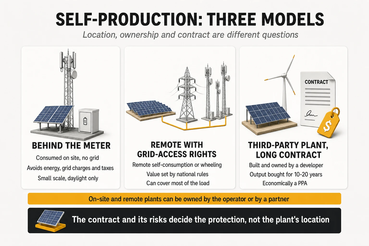
The results are real but rarely expressed in money, and two different problems are being solved. In markets with unreliable grids, solar replaces diesel: MTN Nigeria still drew 58% of its energy from diesel in 2025, with base-station diesel costing more than 60 billion naira a year (Technext), and pass-through power contracts with tower companies create split incentives that slow retrofits (GSMA Mobile Net Zero 2026). In liberalised markets with reliable grids, self-production competes with PPAs: behind-the-meter solar avoids the energy price and the variable charges on the energy it covers, but is small and does not reduce the capacity a site must keep for the night; remote models are worth more than a PPA only where regulation lets them avoid charges a PPA cannot.

Self-generation is still tiny in aggregate: about 2 TWh of the 70 TWh of renewable electricity operators used in 2024 (GSMA Mobile Net Zero 2026).

13. What “100% renewable” really means

An operator can report 100% renewable electricity and still be fully exposed to wholesale prices. The renewable claim and the price protection are produced by different instruments, and confusing them is one of the most common errors in board discussions about energy.

Approach	What it means	Price protection	Time matching	Contribution to new capacity
Unbundled certificates (guarantees of origin, RECs, I-RECs)	The operator buys certificates matching its annual consumption, separately from the energy	None	Annual	Low: certificates are cheap and plentiful
Green tariff from a retailer	The supplier bundles certificates with the energy supply	Only what the supply contract fixes	Annual	Low to moderate
Renewable PPA	Long-term contract linked to specific plants	High for the contracted volume and profile	Depends on the profile; often annual	High when the contract finances a new plant; low with existing plants
Hourly (24/7) matching	Consumption matched with clean generation hour by hour	Depends on the instruments used	Hourly	Depends on whether new or existing plants are used

Caption: Four ways to support a renewable electricity claim. Price protection, time matching and contribution to new capacity are three different criteria; no instrument maximises all of them by itself.

Certificates are cheap because they are abundant. European guarantees of origin traded at around 7-10 €/MWh in 2023 and then collapsed below 1 €/MWh for next-year delivery by the end of 2024 (Future Energy); public auctions in Slovakia in 2026 cleared between 0.60 and 1.95 €/MWh (OKTE). That makes them an inexpensive way to report renewable consumption, and a weak signal for new investment. Deutsche Telekom’s 100% renewable claim, for example, rested on 44% guarantees of origin at group level and 70% in Germany in 2024 (Deutsche Telekom), which is fully compliant with current reporting rules and says little about price risk.

Hourly matching and additionality are different things. A portfolio matched hour by hour with output from existing hydro or wind plants is temporally precise but adds no new capacity; a PPA that finances a new solar farm adds capacity but may be matched only annually. Buyers should state which of the two they are pursuing.

The accounting rules may tighten, but slowly. The GHG Protocol consulted in 2025-2026 on a revision of its Scope 2 guidance that included hourly matching; only about 22% of respondents supported making it mandatory, and the board asked for several reporting approaches rather than one rule, with a final standard not expected before 2027-2028 (pv magazine). No operator has yet committed to network-wide hourly matching; NTT Docomo has trialled it at selected sites using solar and biomass (IT Business Today).

For energy management, the implication is practical. The renewable claim should be a by-product of a procurement strategy designed for cost and risk, not the other way round. A PPA portfolio built to serve the hourly load at a stable price will also deliver a credible renewable claim; a certificate portfolio built to report 100% renewable will not protect the P&L from the next gas spike.

14. The operating model: running energy as a portfolio

In a large operator, energy cannot be a line item managed by a buyer who runs a tender every three years. It needs a permanent capability — an energy desk — that combines market, network, finance and data skills, and that reports to someone who owns the full cost.

Capabilities and KPIs of the energy function

Capability	What it manages	Main KPI
Demand forecasting	Hourly consumption by site cluster, technology and region, including decommissioning and growth plans	Forecast error (% of annual GWh and hourly MAPE)
Market intelligence	Spot and forwards, gas, carbon, hydro, outages, regulation	Scenario cost range for the next 36 months
Structural contracting	PPAs by technology, tenor, volume and profile	Average cost of the core layer; renewal coverage
Tactical hedging	Tranches, clicks, hedge ratios by year	Hedged share vs policy by delivery year
Risk management	Budget at risk, counterparty exposure, credit support	Budget at risk vs approved limit
Supply optimisation	Contracted capacity, tariffs, reactive energy, invoice validation	All-in €/MWh by perimeter; overcharges recovered
Efficiency coordination	Decommissioning, modernisation, cooling, data centres	GWh saved vs plan; € saved at marginal cost
Monetisation	Government efficiency incentives, flexibility revenues	Net cash realised (not issued or estimated)
Reporting and claims	Certificates, renewable share, Scope 2	Audit-ready renewable and emissions data

Caption: The capabilities of a telco energy desk and the KPI that measures each one.

Governance: who decides what

The market function proposes; finance decides the risk; the network executes the demand side. A workable model has four elements: an energy risk policy approved by the CFO or the board (hedge-ratio bands, budget-at-risk limits, eligible instruments, counterparties, delegations); an energy committee with procurement, treasury, network operations, sustainability and accounting, meeting monthly and more often in a crisis; a single demand scenario shared by the network and procurement plans; and, as in any treasury, separation between the person who buys and the person who reports the result.

The energy cost bridge

The most useful management tool is a bridge that explains why the forecast energy cost has moved since the budget. Each bar isolates one driver: the price effect on the open volume, the volume effect (decommissioning delays, growth, weather), the effect of hedges executed at prices different from the budget, system and network charges, efficiency savings valued at marginal avoided cost, and incentive income recognised under the agreed accounting rules.

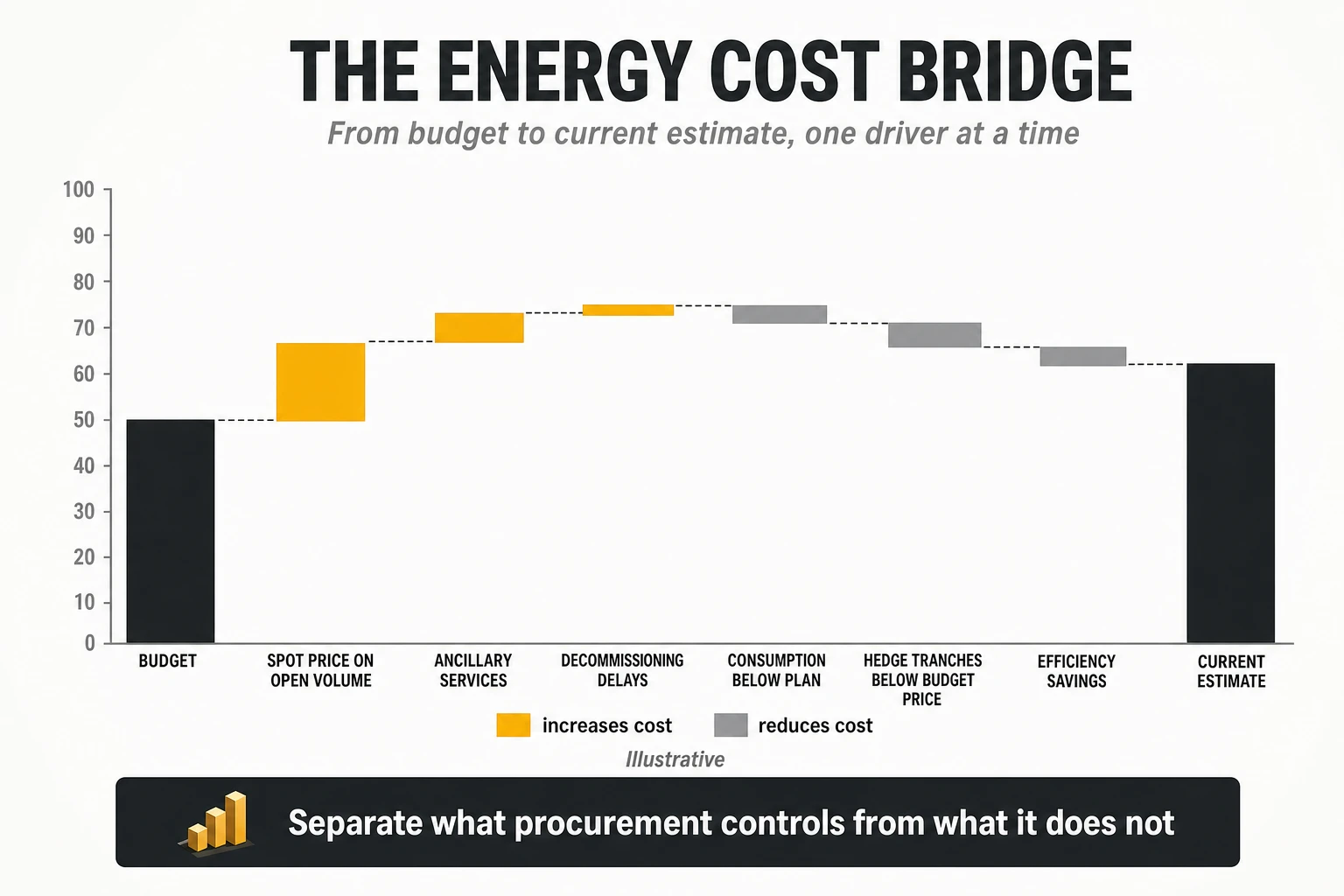
A bridge like this changes conversations. When the estimate rises by 25 M€ in a quarter, the committee can see that, for example, 18 M€ come from spot prices on the open volume, 5 M€ from ancillary services and 2 M€ from a delayed decommissioning programme — and act on each separately.

Where analytics and AI help

Advanced analytics adds real value in four places: hourly demand forecasting by site cluster; anomaly detection across tens of thousands of meters (sites consuming when they should be off, capacity contracted for equipment that no longer exists); RAN energy optimisation; and portfolio models that combine hourly demand, existing contracts, forward curves and risk limits to recommend which volume to hedge, for which years, with which products.

What AI should not do is trade. The output of any model should be a traceable recommendation that the energy committee approves under the risk policy.

15. After the hedge cliff: six strategic options

Every large operator with legacy PPAs will face the same question within this decade: how to replace cheap protection that is expiring without locking itself into expensive contracts or leaving too much volume exposed. There are six broad options. They are not mutually exclusive, and they should be judged with the same yardstick as the strategy comparison in section 8: cost of serving the hourly load, and cost in a crisis.

Option	What it means	Effect on price risk	Effect on cost level	Main limitation
1. Roll the programme passively	Renew PPAs and hedges as they expire, with the same policy and products	Maintains protection, at the market price of the renewal year	Higher than the legacy contracts	Inherits whatever the market offers at that moment
2. Stagger and diversify hedges	Start renewals three to five years ahead, split them into tranches, mix tenors, use collars	Smooths the cliff; avoids buying everything at one price	Neutral to slightly higher	Requires credit lines, a risk policy and discipline
3. Shape-aware long-term contracts	New PPAs chosen on cost to serve the load: solar-wind mixes, hybrids with storage, baseload products, including plants built for the operator by third parties	Strong for the contracted volume and profile	Depends on product and market; usually above solar headline prices	Long commitment; volume must match the demand plan
4. Self-production where the rules reward it	Behind-the-meter generation, and remote self-consumption or wheeling where available	Covers part of the volume and avoids some grid charges	Competitive where the regulation lets it avoid charges	Small behind the meter; remote models depend on national rules
5. Own or co-own generation	Equity stakes in plants, or long-term tolling agreements	Strong, beyond usual PPA horizons	Potentially low over the asset life	Capital, non-core risk, balance-sheet impact
6. Storage and flexibility	Batteries at sites and data centres for peak shaving, arbitrage and grid services	Reduces exposure to peak hours	Moderate; revenue depends on market rules	Small relative to total load; battery wear and backup needs

Caption: Six strategic options to replace expiring energy protection. A third-party plant bought under a long-term contract belongs to option 3: economically, it is a PPA.

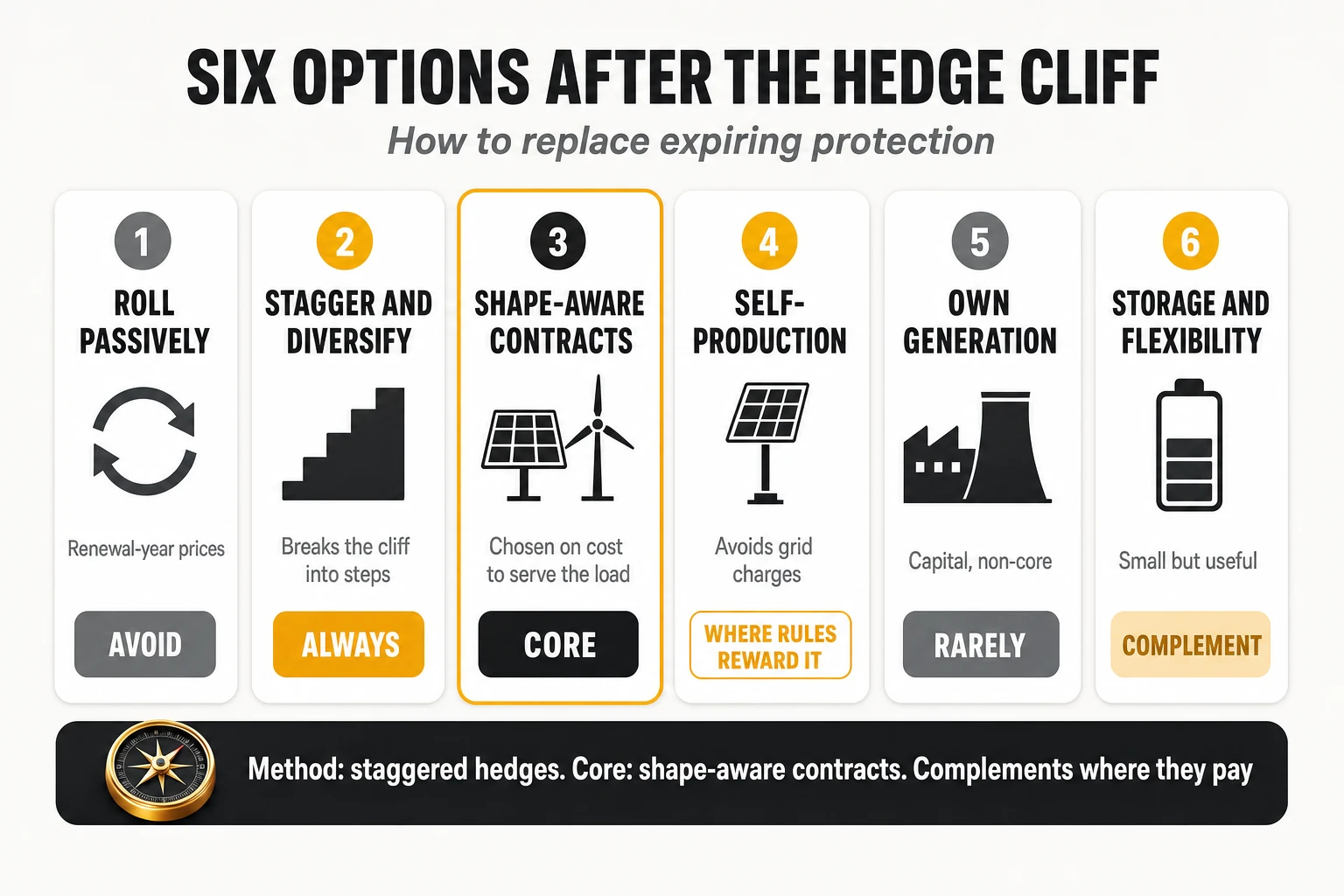
Our assessment

Under the conditions of most large operators in liberalised markets, the combination that looks most robust is option 2 as the method, option 3 as the core, option 4 where regulation rewards it and option 6 as an incremental revenue line, all sized against a demand plan that already includes decommissioning. Option 1 is the most dangerous if applied passively, because it renews concentrated volumes at the renewal year’s prices, often with a solar-heavy profile that served well when the night-time spread was smaller. Option 5 rarely makes sense for a telco, whose balance sheet is already stretched by fibre and spectrum. The worst outcome is to let the cliff arrive with no decision, which is still the most common one.

16. The playbook: how an operator anticipates and controls energy cost

An operator cannot forecast the next war, drought or cold spell. It can decide in advance how it will review the situation when the signals appear, who decides and within which limits, so that decisions are taken calmly and with the full picture. This section brings the previous ones together into a practical playbook.

What the operator can actually control

The cost of energy is the product of five things, and the operator has a lever on each.

What drives the cost	Lever	Owner
Price of the energy	Hedge ratio, timing of tranches, contract structure, product mix	Procurement, with risk limits set by finance
Volume	Decommissioning, modernisation, efficiency, data centre consolidation	Network operations and technology
Shape (when energy is consumed)	Shape-aware contracts, storage, peak shaving, flexible loads	Procurement and operations
Non-energy parts of the bill	Contracted capacity, voltage level, tariffs, reactive energy, invoice validation, tower-company pass-through	Energy management and operations
Contract terms	Volume flexibility, negative-price and change-in-law clauses, termination and assignment rights	Procurement and legal

Caption: The five components of energy cost and the levers that control each one.

An early-warning system: signals that trigger a review, not a purchase

Anticipation means deciding in advance which signals deserve attention, who reviews them and how fast. A crossed threshold does not mean “buy”. By the time an alarming indicator is public, forward prices usually reflect it, and buying then may lock in the risk premium rather than avoid it. A threshold triggers a structured review: what the market now prices, how much is already hedged, what the residual exposure costs in each scenario against the budget, and which responses the risk policy allows. The thresholds below are examples; each operator calibrates its own.

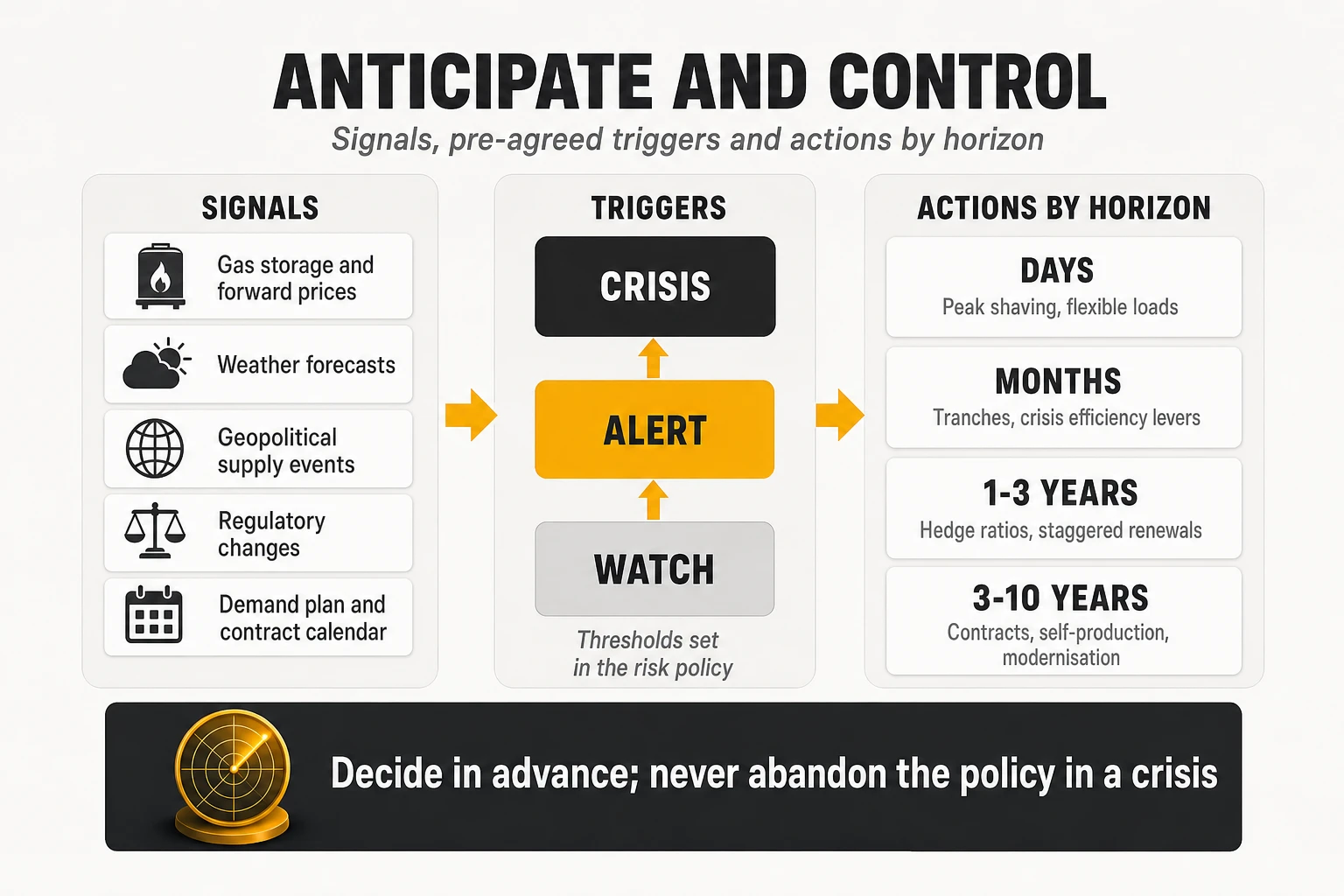
Signal	Example threshold	Review and possible responses within the policy
Gas storage going into winter	More than 10 points below the five-year average in October	Re-run winter scenarios; compare the cost of extra cover at current forward prices with the budget at risk; check that crisis demand levers are ready
Forward prices rise sharply	Next-year forward up more than 25% in a month	Keep executing time-based tranches; avoid accelerating purchases at the peak; recalculate budget at risk; inform the CFO; prepare demand levers
Forward prices fall	Y+2 or Y+3 forward below the target price set in the policy	Consider accelerating tranches for those years within the maximum band; open PPA discussions
Hydro reserves (hydro-heavy systems)	Usable reserves well below average at the end of the wet season	Re-run summer and autumn scenarios; assess whether the forward curve already reflects the shortfall
Geopolitical supply event	Disruption of a major gas or LNG route, sanctions, attack on infrastructure	Energy committee within 48 hours; stress test with gas doubled; decide whether to move to the “alert” stage
Weather forecast	Cold, calm, overcast week; heatwave	Peak shaving with site batteries; postpone flexible loads; check cooling set points
Interconnection or plant outages	Long outage of an interconnector or large baseload plants	Review short-term exposure for the affected months
Regulatory change	Proposal to change network tariffs, levies or market rules	Model the impact; check change-in-law clauses; respond to consultations
Demand plan deviation	Decommissioning delayed or accelerated by more than a quarter	Adjust hedged volume up or down; use volume bands or resale rights
Contract calendar	A PPA or block expiring within five years without a replacement plan	Start the renewal process; include it in the hedge-cliff plan

Caption: Examples of signals, thresholds and responses. A threshold triggers a review against current prices, existing hedges and residual exposure; the response is decided within the energy risk policy.

A three-stage crisis protocol

A crisis is not the moment to design governance. A simple protocol, approved in advance, defines who does what as conditions worsen.

1. Watch. Normal weekly routine: indicators, scenarios, triggers, tranches according to policy. Crisis levers are inventoried and tested once a year.
2. Alert — triggered by a supply event, a sharp rise in forwards or a budget-at-risk threshold. The energy committee meets more often; the year-end estimate is updated more frequently; demand levers are prepared; next-year hedging is reviewed against the risk policy, with current forward prices in view; tower companies and large hosting providers are asked for their own exposure.
3. Crisis — triggered by spot prices far above budget for several weeks. Demand levers are activated, valued at the market price of the open volume; flexibility contracts and peak shaving are used; the executive committee receives the cost bridge regularly; pricing and budget decisions are escalated; and, crucially, the hedging policy is not abandoned — buying years of volume at crisis prices is how a temporary shock becomes a permanent cost.

Levers by time horizon

The shorter the horizon, the more the operator depends on demand-side levers; the longer, the more it can shape price and structure. Within days, only consumption can move — peak shaving, flexible loads, cooling set points. Within months, tactical tranches and crisis efficiency levers act on this year’s and next year’s open volume. Over one to three years, hedge ratios, staggered renewals and decommissioning set the price of most of the volume. Over three to ten years, long-term contracts, self-production and network modernisation set the structure of the portfolio.

Priorities by type of operator

The principles are universal; the priorities are not. The same toolbox produces very different programmes depending on the market structure and the operator’s position.

Operator profile	Main energy risk	Priority levers	What to avoid
Large incumbent in a liberalised market (Europe, Australia, parts of North America)	Hedge cliff as legacy PPAs expire; growing system charges	Early, staggered renewals; shape-aware PPAs; legacy decommissioning; government efficiency incentives	Concentrated renewals; solar-only portfolios
Challenger or mid-size operator	Lack of scale to sign PPAs; full exposure to retail prices	Multi-buyer PPAs, retailer clicking rights, tight capacity and invoice management	Long contracts sized on optimistic growth
Operator in a nodal market (most of the US)	Basis risk between project node and consumption	Settlement at liquid hubs; regional diversification; hedge accounting set up early	VPPAs settled at remote nodes without basis analysis
Operator in a regulated or single-buyer market	Tariff increases; grid unreliability; diesel cost	Solar-hybrid sites, energy-as-a-service with tower companies, efficiency	Applying European hedging playbooks where no market exists
Operator that sold its towers	Energy re-invoiced by tower companies with limited visibility	Contractual transparency, pass-through audits, joint efficiency programmes with the towerco	Treating re-invoiced energy as outside the energy strategy
Operator with fast-growing data centre or AI load	Consumption rising faster than efficiency cuts it	Dedicated procurement for data centre load, 24/7 products, location strategy	Using network efficiency gains to mask data centre growth

Caption: Energy priorities by operator profile.

A twelve-month plan to get started

1. Months 1-3 — Know the position. An inventory of every PPA, hedge and supply contract (hourly volume, price, tenor, settlement point, exit clauses, counterparty) and the three-level cost reconciliation, giving the marginal value of a saved MWh under each contract.
2. Months 2-5 — Set the rules. An hourly demand model with plan, delay and acceleration scenarios agreed with the network organisation, and a risk policy with hedge-ratio bands, budget-at-risk limits and governance approved by the CFO.
3. Months 4-8 — Plan the cliff and take the quick wins. A staggered renewal calendar with products chosen on cost to serve the load; contracted-capacity review, invoice validation, idle sites, cooling set points.
4. Months 6-12 — Launch the structural programmes. Decommissioning acceleration, RAN energy features, self-production where the rules reward it, the efficiency incentive pipeline and a flexibility pilot.
5. Month 12 — Report. The first full cost bridge to the executive committee, with the hedge-cliff chart on the first page.

17. Conclusions

Energy in a telco is no longer a utility bill; it is a portfolio. A continuous network load meets a market whose price in the hours the network cannot avoid is often set by gas and moved by weather and geopolitics, through contracts that last longer than most network technologies, while the operator itself reshapes its demand through decommissioning and growth.

Four ideas matter most.

• Judge every contract by the cost of serving the load, in every scenario. A 35 €/MWh solar PPA can cost 85 €/MWh in practice; in a one-year example, flat and diversified portfolios cost almost 40% less than the market in a crisis, at a premium of about 2 €/MWh of expected cost against the cheapest diversified option.
• Treat procurement and consumption as one plan. The value of switching equipment off depends on the contract that bought its energy, and the volume of new contracts depends on the decommissioning plan.
• Start renewing before the cliff. Long-term contracts signed before 2022 are expiring; staggered, shape-aware renewals started years ahead are the cheapest protection available.
• Make anticipation a policy. Signals and thresholds should trigger a disciplined review within agreed limits — neither paralysis nor panic buying.

The operators that will have the lowest energy cost in 2030 are not those that sign the cheapest PPA this year. They are those that know, hour by hour and contract by contract, what their network consumes, what it costs and what is protected — and that use the time their hedges buy to reduce consumption and renew their protection before the market forces them to.

---

At TelcoCrux, we analyse the decisions that shape an operator’s cost base, and energy is becoming one of the most consequential. If you are working on these questions — a hedge cliff approaching, a PPA renewal, the link between decommissioning and procurement — and want to compare notes or challenge this analysis, get in touch.