Network Digital Twins on Graphs

1. A network that nobody can draw

At 02:10 on a weekday, the network operations centre (NOC) of a regional mobile operator in the Dallas – Fort Worth area receives 340 alarms in eleven minutes. They come from radio cells in Plano, from two aggregation routers, from a transport ring and from a user plane function in the core. Six consoles show six partial pictures. The questions that matter are simple to ask and hard to answer: is this one fault or several, where did it start, which enterprise customers are affected, and is anything else about to fail because of it?

Every piece of evidence needed to answer is already collected. The alarms are in the fault manager, the counters in the performance system, the topology in two inventory databases that disagree on 4% of their links, the circuits in a third system and the open changes in the ticketing tool. What is missing is not data. It is a single, current model that joins those sources and can be asked a question that crosses them: what depends on what, right now.

That model is what the industry has started to call a network digital twin. The term is overloaded. It is used for 3D renders of radio propagation, for configuration verification tools, for planning simulators and for vendor dashboards. This article uses it in the narrow, operational sense that matters for assurance: a live, queryable graph of what the network is, what state it is in and what depends on what, joined to its history and to the models that reason over it.

The thesis is straightforward. A network digital twin earns its cost when it gives observability the context it lacks: an address for every symptom, a dependency chain for every fault and a memory of what happened before. Graph technology makes that model natural to store and fast to query. The hard part was always building it, and that part has changed: AI-assisted modelling can now turn a folder of flat inventory exports into a first ontology in weeks rather than quarters. It does not remove the engineering review, the ongoing data feeds or the obligation to prove that the twin answers something the operator’s existing deterministic tools cannot. And the choice of platform is less binary than it looks: the two approaches operators most often shortlist — Google’s integrated stack around Spanner Graph and Neo4j’s specialised graph ecosystem — lead in different places and can even be combined.

The article moves from concept to product to practice.

Sections 1 to 3 define the twin, explain why a telecom network is naturally a graph and show precisely how the twin complements monitoring and observability.
Sections 4 and 5 describe a vendor-neutral architecture and the five families of products sold under the same name.
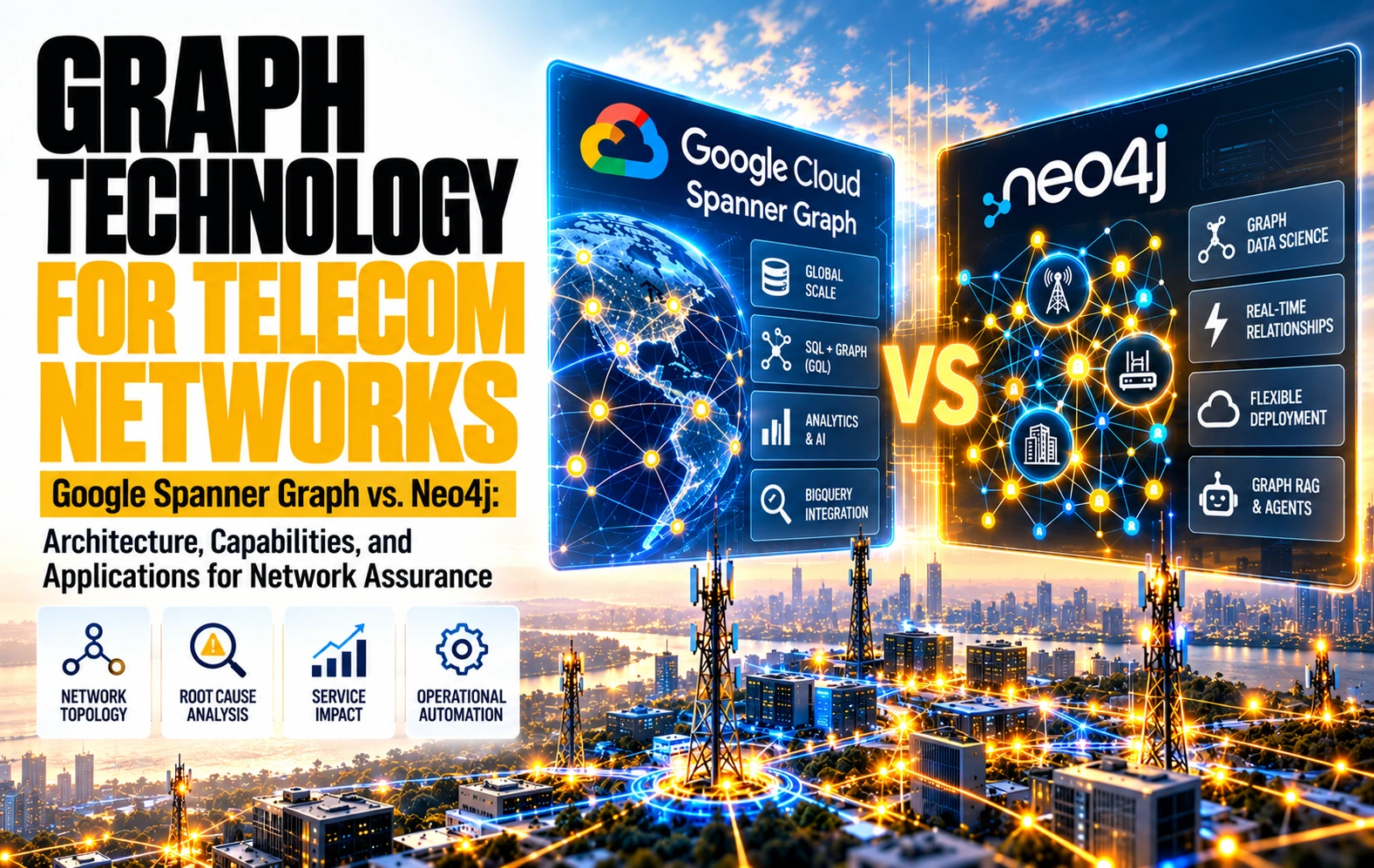
Sections 6 and 7 examine, at the same depth, the two approaches that operators most often shortlist for the operational twin: Google Cloud’s integrated stack (Spanner Graph, BigQuery, its AI platform and agents) and Neo4j’s specialised graph ecosystem (native graph database, Graph Data Science, GraphRAG and agents).
Section 8 covers the step that most changes the economics on either platform: loading the twin from CSV files.
Section 9 compares the two head to head: architecture, scaling, use cases, evidence, cost and three architectures worth evaluating.
Sections 10 and 11 show what the twin can answer once it is loaded, through seven practical cases built on illustrative US data.
Sections 12 to 14 cover the limits, a pilot and benchmark design with kill criteria, and the conclusions.

A note on sources and data. Product capabilities are taken from public documentation, linked in the text. The seven practical cases use fictional identifiers and US locations to illustrate typical operational patterns; they are not measurements from a named operator, and every figure in them is labelled as illustrative. Assessments of strengths and limits are TelcoCrux views.

What the term means, in three levels

The most useful classification of digital twins comes from manufacturing research, not from telecom marketing. Kritzinger and co-authors (2018) separated three levels by the direction in which data flows between the physical system and its digital copy. The distinction translates directly to networks and removes most of the ambiguity in vendor presentations.

Digital model. A static representation of the network: inventory and topology, connected, but updated by hand or by periodic batch. It answers structural questions — the possible paths between two nodes, the single points of failure, the elements that share a duct or a power feed.
Digital shadow. The model kept current automatically by a one-way flow from the network: alarms, performance counters, configuration and logs attached to the entities they describe. It answers operational questions — the latency and spare capacity between A and B now, the over- and under-used paths, the probable root cause of an anomaly.
Digital twin. The shadow plus a return path: simulation and prediction good enough to evaluate a change before it is made, and a validated route back into the network through controllers. It answers what-if questions — what happens if this routing table changes, how would yesterday’s traffic behave on a modified topology.

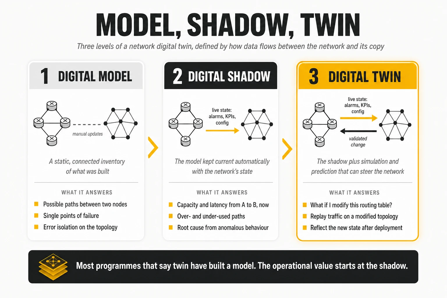
Model, shadow, twin: three levels defined by how data flows between the network and its copy. Most programmes that announce a twin have built a model; the operational value for assurance starts at the shadow.

The practical consequence is that most operators should aim for a shadow first. A model without live state is an inventory with a better query language. A full twin needs simulation fidelity that few domains have yet, and a closed loop that few operators will authorise without a long track record. The shadow is where root cause analysis, impact assessment and agent grounding become possible, and it is the level at which every case in section 11 operates.

What the standards bodies say

Two reference documents give the concept a vendor-neutral shape. The ITU-T approved Recommendation Y.3090, Digital twin network — Requirements and architecture, in February 2022. In the IRTF, the Network Management Research Group’s draft Network Digital Twin (NDT): Concepts and Reference Architecture (revision 13, July 2026, informational and not yet an RFC) defines a network digital twin through four key elements:

Data: the repository of network state, configuration, topology and history that the twin is built on.
Models: the functional and behavioural models — of topology, of traffic, of failures — that turn data into answers.
Interfaces: the standardised ways in which applications query the twin and in which the twin exchanges data with the real network.
Mapping: the continuous correspondence between each physical entity and its digital counterpart, kept accurate as the network changes.

Mapping is the element that decides whether a twin is useful. A twin whose mapping lags the network by a week will send an engineer to the wrong ring. Every architectural decision later in this article — real-time feeds, a single operational copy, inventory integration — exists to keep the mapping honest.

2. Why a telecom network is naturally a graph

A telecom network is a set of things and the relationships between them, and that is the definition of a graph. Sites host cells, cells are backhauled by routers, routers connect to routers over links that ride on fibre spans, services depend on paths, customers depend on services. A graph database stores exactly that: nodes, edges and the properties attached to both.

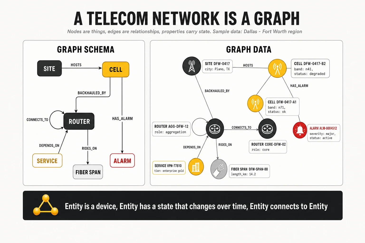
Nodes are things, edges are relationships, properties carry state. The schema on the left is the ontology; the data on the right is the twin. Identifiers and locations are illustrative.

Nodes, edges and properties

Three rules cover most of what a network twin needs to represent. They also explain why the model is easy to describe and hard to build.

An entity is a thing: a device, an antenna sector, a server, a virtual function, a fibre span, a service, a customer site. Each is a node with an identifier and properties such as vendor, software release, location or role.
An entity has states that change over time: alarms, performance samples, configuration versions, tickets, maintenance windows. These are either properties with timestamps or separate nodes linked by edges such as HAS_FAULT or HAS_TICKET, which keeps history queryable.
An entity connects to other entities: physically (CONNECTS_TO, RIDES_ON), logically (BACKHAULED_BY, DEPENDS_ON) or administratively (OWNED_BY, MAINTAINED_BY). The edges are where the operational value lives, because impact and causation travel along them.

A financial example makes the structure familiar. In fraud detection, a person owns accounts, accounts transfer money to other accounts, and an account repays a loan; a ring of transfers between accounts that look unrelated is invisible in a table and obvious in a graph. In a network, the equivalent of the fraud ring is the failure that propagates through three layers and surfaces as symptoms in places that look unrelated.

Why not simply use relational tables?

Relational databases can store the same information; they struggle to query it at depth. A question such as “every service within four hops of this router that has an active major alarm” requires a chain of self-joins or a recursive query whose cost grows with every hop and whose text quickly becomes unreadable. A graph query expresses the same question as a pattern — a node, a path of up to four CONNECTS_TO edges, a node with a HAS_FAULT edge — and the engine is built to traverse it.

The query language has also become a standard. In April 2024, ISO and IEC published ISO/IEC 39075, GQL, the first new ISO database query language since SQL, for property graphs. Its companion, SQL/PGQ (ISO/IEC 9075-16:2023), adds property-graph queries inside SQL. Standardisation matters for an operator choosing a platform for a decade: queries written in a standard language are less of a lock-in than queries written in a product dialect.

Four layers of graph technology: from network context to predictive intelligence

“Graph” is used for four different things, and separating them is the key to the rest of this article. They are layers of capability, not four products to install: each builds on the one below, and each can be supplied by different tools.

The graph model, or knowledge graph. The representation itself: entities, their relationships and what they mean — cell to router to transport ring to service to customer. It is a design artefact; it can exist in a spreadsheet, a set of relational tables or a dedicated database.
The graph database. The engine that stores the model and answers questions over it: which services depend on this router, what is within four hops, what has changed. Neo4j, Google Spanner Graph and Amazon Neptune are examples.
Graph analytics, or graph data science. Algorithms that compute properties of the whole structure rather than answering one question: which routers are most central, which nodes or links would split the network if lost, which elements form tightly connected clusters, which path has the lowest cost. The results are deterministic and reproducible.
Graph neural networks (GNNs). Machine learning models that learn from the attributes of nodes and the way they are connected. Trained on thousands of past incidents, a GNN can learn how degradations propagate between related elements and predict the probable origin of a new one, or which element is likely to fail next.

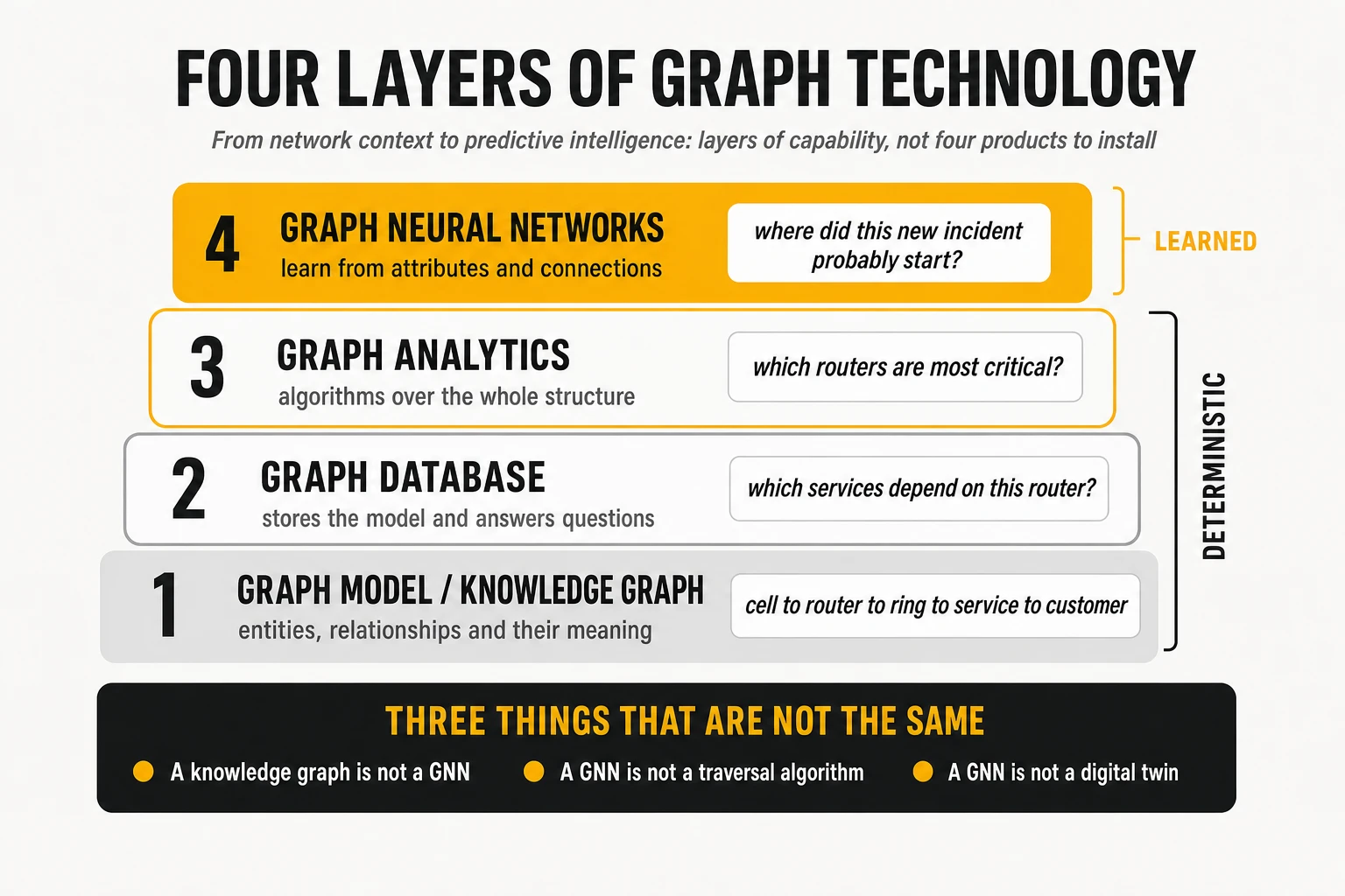
Four layers of graph technology. The first three are deterministic and deliver most of the value for network assurance; the fourth adds learning, and with it the need for training data, validation and monitoring.

A network of 100,000 elements and millions of relationships shows the difference. The database answers which services depend on a given router. Graph analytics computes which routers are most critical because of how they are connected. A GNN learns from historical incidents how problems spread through those connections and suggests where a new incident probably started. The first two are entirely deterministic; the third requires training, adequate historical data and validation, and its answers come with a confidence, not a certainty.

Three distinctions prevent the most common misunderstandings.

A GNN is not another traversal algorithm. An algorithm computes a defined property of the graph; a GNN learns a function from examples. And it does not have to run inside the database that stores the graph: the graph is typically exported or read into a machine learning platform, trained there, and the predictions are written back.
Having a knowledge graph does not mean having a GNN, and most of the value of a twin comes before any neural network is trained.
Having a GNN does not mean having a digital twin. A twin also needs live state, the mapping to the real network and, eventually, a return path into it.

Both platforms examined later cover all four layers, with different products and different maturity.

Layer	Google Cloud	Neo4j
1. Graph model	Defined by the operator, expressed as tables and a property graph schema	Defined by the operator, expressed as node labels, relationship types and graph types
2. Graph database	Spanner Graph	Neo4j Database or AuraDB
3. Graph analytics	Spanner Graph algorithms (preview in October 2026)	Graph Data Science, largely production-grade
4. Graph neural networks	Distributed Graph Flow, TensorFlow GNN and Google’s ML platform	GraphSAGE embeddings in GDS (beta) and external frameworks such as PyTorch Geometric
Agents on top	Gemini, Agent Development Kit	GraphRAG, Aura Agent, MCP

The four layers on each platform. Neither supplies layer 1: the model of the network is always the operator’s work.

This article treats GNNs as an advanced AI capability on top of the graph — not as a database, and not as an alternative to Neo4j or Spanner. The four layers explain both the deterministic applications that already pay for a twin in network assurance and the later step towards predictive and autonomous operations.

The ontology question: why no one sells a telco model that just fits

The schema of a twin — its ontology — is where operators expect a vendor to arrive with an answer, and where none does. The industry has partial models: the TM Forum’s information framework for services and resources, 3GPP network resource models for mobile functions, IETF YANG models for configuration, ONF’s transport API for optical and packet transport. Each covers a slice. None reflects the way a specific operator has named, split and joined its inventories over twenty years.

The consequence is unavoidable: the operator has to define what a tunnel, a virtual router or a service instance means in its own systems, and the loading pipelines have to be written against its own sources. Even where two operators buy from the same equipment vendors, each inventory has its own conventions, exceptions and missing keys. The realistic expectation is a reusable method and reusable patterns, not a reusable ontology. Section 8 shows how much of the method can now be automated, and what cannot.

3. How the twin complements observability

Observability and the twin answer different questions, and confusing them is the most common design error. Observability — metrics, logs, traces, events, streaming telemetry, probes and quality-of-experience measurements — tells the operator what is happening. The twin tells it what that evidence is connected to: which element, on which path, under which service, for which customer, after which change. One supplies evidence; the other supplies context and memory.

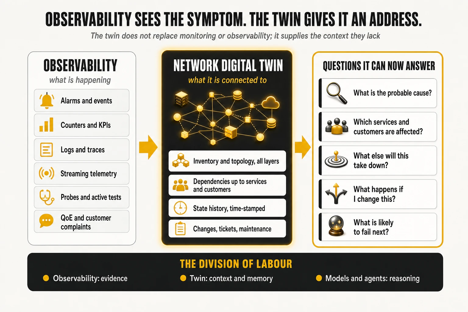
Observability sees the symptom; the twin gives it an address. The twin does not replace monitoring or observability tools: it supplies the context that turns their evidence into answers.

The division of labour, question by question

The difference is easiest to see in the questions a network operations centre actually asks.

Operational question	Observability alone	With a graph-based twin
Is this one fault or several?	Correlation by time window and text similarity; topology guessed from naming conventions	Correlation along real dependency edges; alarms that share an upstream element collapse into one incident
Where did it start?	The earliest or loudest alarm, often a symptom	The deepest common ancestor in the dependency chain, ranked with evidence from each layer
Who is affected?	Inferred later from complaints and tickets	A traversal from the faulty element up to services, enterprise sites and their service-level agreements (SLAs), computed in seconds
What else will this take down?	Not answerable until it happens	Elements that lose redundancy because of this fault: the single points of failure that now exist
What happens if I change this?	Not answerable	Paths, services and customers that depend on the element to be changed, before the change window opens
What is likely to fail next?	Threshold breaches and trend lines per counter	Patterns across connected elements, learned from history, including degradations that never raised an alarm

The same six questions with and without a twin. Observability supplies the evidence in every row; the twin supplies the relationships that make the right-hand column possible.

The previous TelcoCrux analysis of end-to-end assurance placed this context in a dedicated shared layer. In that reference architecture, network and service context — discovery, federated inventory, multilayer topology, a temporal knowledge graph and the chain from resource to commitment — is layer 07, and it feeds the diagnosis block (02: correlation, root cause, impact) and the agentic layer (08). A graph-based twin is one concrete way to build layer 07 and expose it to the rest. This article goes inside that layer.

Determinism first, learning second

A fair objection is that many of these questions are already answered deterministically. When a fibre ring is cut, a topology-aware correlation engine walks the known dependencies and names the span with near certainty; no neural network is needed, and none should be paid for. Operators that already run graph-based correlation for their IP and transport layers — several do, on general-purpose graph databases — have solved the textbook cases.

The case for adding statistical and learned models rests on the cases determinism cannot reach.

Silent failures: degradations that never cross a threshold, visible only as a statistical shift in a group of connected elements.
Cascades under load: an event — a championship game, a holiday exodus on an interstate, a weather front — that produces a chain of performance problems in cells not adjacent to the event, through backhaul and core dependencies.
Ranking under uncertainty: several plausible origins, where the useful output is a ranked list with confidence and business impact, not one answer.
Prediction: which element is likely to fail next, given the pattern of what failed before in similar parts of the graph.
What-if: the effect of a change or of a predicted event before it happens.

The economic test is therefore narrow and should be applied honestly. If a deterministic rule on the graph answers the question, use the rule; it is cheaper, explainable and already trusted. Between simple rules and learned models sits a middle ground that is often overlooked: graph algorithms — centrality, articulation points, bridges, communities — which are deterministic mathematics and reveal structural weaknesses no inventory shows. Learned models earn their cost only where both run out, and the pilot design in section 13 is built to measure exactly that difference.

What a twin does not do

Three expectations cause disappointment and are worth removing early.

A twin does not discover the network by itself. It reflects its sources. If a new router is installed and no inventory, controller or discovery feed reports it, the twin will not know. “Real time” means that whatever the sources report is reflected immediately, not that the twin observes the network directly.
A twin is not automatically the system of record. It can hold the inventory, and for parts of the estate with no inventory it may become the first one, but most operators integrate it with existing inventory systems rather than replace them.
A twin is not plug-and-play. Defining the entities, writing the feeds and keeping the mapping accurate is a non-trivial effort that sits with the operator, even when tools accelerate it. Presenting it otherwise to an executive sponsor is the fastest way to lose the programme in its second quarter.

4. Anatomy of a graph-based twin, independent of any vendor

Before looking at any product, it helps to fix the architecture that every credible implementation converges on. It has five layers and one transversal concern, and the decisions that matter are about where each kind of question is answered and how many copies of the topology exist.

A vendor-neutral reference architecture. Real-time questions go to the operational graph; questions about history go to the warehouse; models and agents sit on top of both, under one governance layer.

Sources and feeds: the twin is only as current as its slowest feed

The twin consumes five kinds of source, and each has a different natural rhythm.

Inventory and configuration management: physical and logical inventory, circuits, the configuration management database (CMDB), usually held in the operations support systems (OSS). Changes are relatively rare and should arrive as events, not nightly dumps.
Controllers and element managers: the most accurate view of the current topology for the domains they manage, usually exposed through northbound APIs.
Fault and performance: alarms, counters, key performance indicators (KPIs) and streaming telemetry. Volumes are high; the twin needs current state and a pointer to history, not every sample.
Operational records: incidents, trouble tickets, change requests and maintenance windows, which give the twin its memory of human activity.
Reference data: site coordinates, address and customer mappings, service catalogues and contractual commitments.

On-premises collection is usually unavoidable. Element managers and controllers sit inside the operator’s network; a gateway layer handles secure ingestion of streams, real-time event processing and, where the twin is allowed to act, a controlled path for configuration through a jump host. The design question is not whether this gateway exists but how thin it can be.

Two stores, by design: operational and analytical

A telecom network can produce terabytes of fault, performance and log data per day, and that does not belong in the database that answers a traversal in milliseconds. Every serious architecture therefore separates two stores and connects them deliberately.

The operational store holds the current topology, current state and recent events as a graph. It serves low-latency, granular queries: neighbours, paths, blast radius, the state of one element now. It is the single current copy of the network model.
The analytical store is a data warehouse holding years of history: KPIs, alarms, tickets, aggregated features. It serves large aggregated queries, training data for models and reporting, at a much lower storage cost per terabyte.

The connection between them is where implementations differ most. Change data capture streams every update from the operational store into the warehouse so history accumulates without batch jobs; reverse ETL (extract, transform, load in the opposite direction) pushes computed results — risk scores, predicted loads, insights — from the warehouse back into the operational graph where agents can use them; and federated queries let analysts join both without copying. The fewer hand-written pipelines in this loop, the longer the twin stays accurate.

One engine with several models, or one engine per model

A twin needs more than graph traversal. A realistic question combines several access patterns: “is there any incident mentioning fibre in the last thirty minutes near Plano, on an element within two hops of this enterprise service?” That is full-text search, a time filter, a geographic filter and a graph pattern, possibly with a semantic match on free-text ticket notes.

There are three ways to serve it.

Polyglot persistence: a graph database for topology, a search engine for text, a vector database for semantic search and a relational database for the rest. Each engine is best of breed; each insertion must be propagated to the others; the pipelines between them become a permanent maintenance cost and a source of inconsistency.
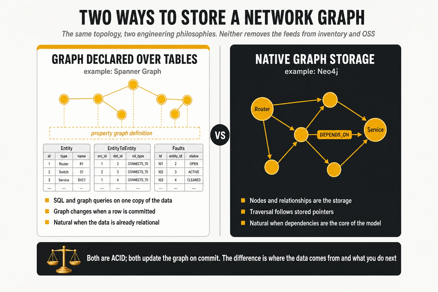
A multi-model relational engine with a graph declared over its tables: one database that supports relational tables, property graphs, full-text and vector indexes over the same rows. Fewer moving parts, one transaction boundary, and SQL and graph on one copy of the data; the trade-off is dependence on one engine’s maturity in each model.
A native graph engine with its own search indexes: nodes and relationships are the storage, and full-text and vector indexes live inside the same database. Traversal is the engine’s speciality; relational data held elsewhere reaches it through connectors.

Two engineering philosophies for the same topology. Both are transactional and both update the graph on commit; the difference is where the data comes from and what the operator does next.

None is correct in general, and the second and third are closer than vendor slides suggest. In both, the graph is current as soon as a transaction commits, with no internal copy to synchronise. What neither removes is the pipeline from the inventory, controllers and fault systems into the database: that integration, not the storage model, is where most of the engineering effort and most of the staleness risk sit. An operator with mature graph databases already in production for parts of its network should not discard them for an architectural preference; an operator starting from scratch should weigh the synchronisation tax of a polyglot design seriously, because it is paid every day for the life of the twin.

Models, agents and governance

Above the stores sit two consumers. Models — forecasting, anomaly detection, graph neural networks, simulation — read the graph and the history and write predictions back. Agents — software components driven by large language models (LLMs) that observe, analyse, decide and, under policy, act — reach the twin through typed, permissioned tools rather than direct database credentials. Governance runs across all of it: identity, policy on what can be read and changed, authorisation proportional to risk, and an audit trail of every query and action an agent performs.

5. Five families sold under one name

“Network digital twin” is used by at least five families of products that solve different problems. Comparing them as if they were alternatives produces bad procurement decisions; most operators will end up running more than one, with the operational twin consuming or feeding the others.

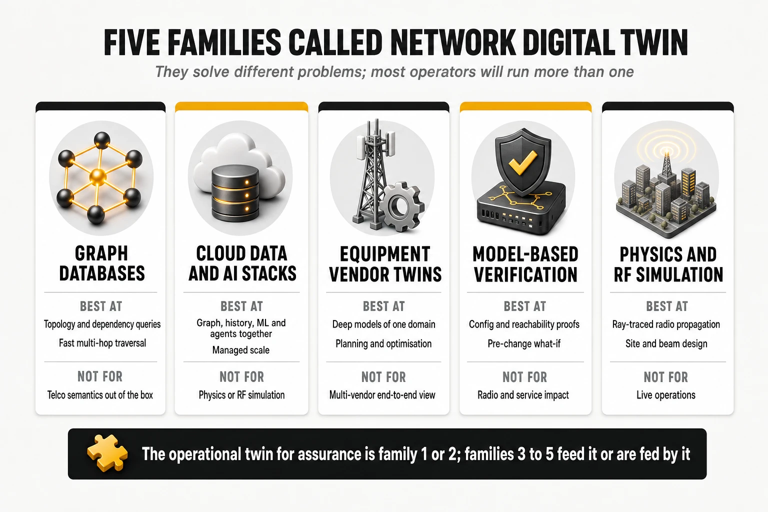
Five families, five problems. The operational twin for assurance is built on families 1 or 2; families 3 to 5 feed it or are fed by it.

Family	What it models	Public examples	Best suited for	Main limit for assurance
1. Graph platforms	Any entities and relationships the operator defines, plus graph analytics and graph-grounded AI	Neo4j (database, Graph Data Science, GraphRAG and agent tooling, section 7) — Comcast has presented a graph-powered digital twin of its nationwide network on it; Memgraph	Topology and dependency queries, structural analytics, correlation over known structure	No telco semantics out of the box; history, warehouse and orchestration are integrated by the operator
2. Cloud data and AI stacks	Graph plus history plus models plus agents, managed	Google Cloud (Spanner Graph, BigQuery and its AI platform, section 6); AWS (Neptune with agentic root cause analysis); Microsoft (Azure Digital Twins and Fabric)	End-to-end operational twin with analytics and AI on one platform	Cloud dependency, data residency questions and the effort of integrating on-premises sources
3. Equipment vendor twins	One domain modelled in depth by its supplier	Nokia RAN Digital Twin and FTTH digital twin; Ericsson Site Digital Twin	Planning, optimisation and deployment within the vendor’s domain	Rarely multi-vendor or end to end; the model belongs to the supplier
4. Model-based verification	Configuration and forwarding state, mathematically	Forward Networks, IP Fabric	Proving reachability and policy before and after a change	Strong on IP and data-centre networks, weak on radio, services and customer impact
5. Physics and RF simulation	Radio propagation and system behaviour, ray-traced	NVIDIA Aerial Omniverse Digital Twin	Site, beam and algorithm design for 5G and 6G	Simulation, not operations; computationally heavy and not fed by live alarms

The market map. Examples are illustrative, not exhaustive, and drawn from public announcements; a presence in a family says nothing about maturity in a given operator’s estate.

Public evidence of operational results is still thin, and should be read accordingly. AWS reports that a network digital twin graph combined with agentic analysis, validated with NTT DOCOMO, isolated failures in transport and the radio access network (RAN) in around fifteen seconds; Google’s partners have shown twins with billions of dependencies in proofs of concept; and TM Forum has reported a temporal twin spanning RAN, transport and core at a large US operator with “up to 35%” projected operations and maintenance savings — a projection, not a measured result. Planning-oriented twins are older: AT&T described in 2022 a network digital twin used to compare the current and next state of its network against resiliency rules. None of this is yet the kind of before-and-after evidence that should be used as a planning assumption.

How to choose between the families

Three questions settle most of the choice.

What is the first decision the twin must improve? Root cause and impact in operations point to families 1 or 2; pre-change verification of IP configuration points to family 4; radio design points to families 3 and 5.
Where must the model live? An operator that wants to own its network model across vendors should not let it live inside one equipment supplier’s tool; families 1 and 2 keep the model in the operator’s own data estate.
What already exists? If graph databases already run correlation for some layers, the question is how to extend or federate them, not how to replace them; the debate between engines is a technical one, not a functional one.

6. Google Cloud’s approach, piece by piece

Google Cloud packages its offer for operators as the Autonomous Network Operations framework, announced in June 2025. It is not a single product. It is a reference design and a set of practices for assembling Google Cloud services around a network digital twin, explicitly modular so that an operator can adopt one layer — for example the twin alone — and keep its existing tools for the rest. The framework document names Spanner and Spanner Graph as the real-time twin, BigQuery as the analytical store, Gemini models and graph neural networks for reasoning and prediction, multi-agent systems on top, and partners including Amdocs, Ericsson and Nokia.

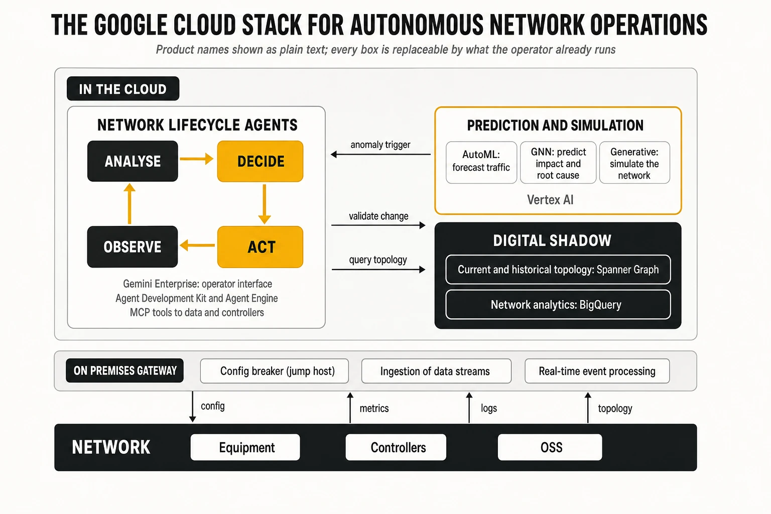
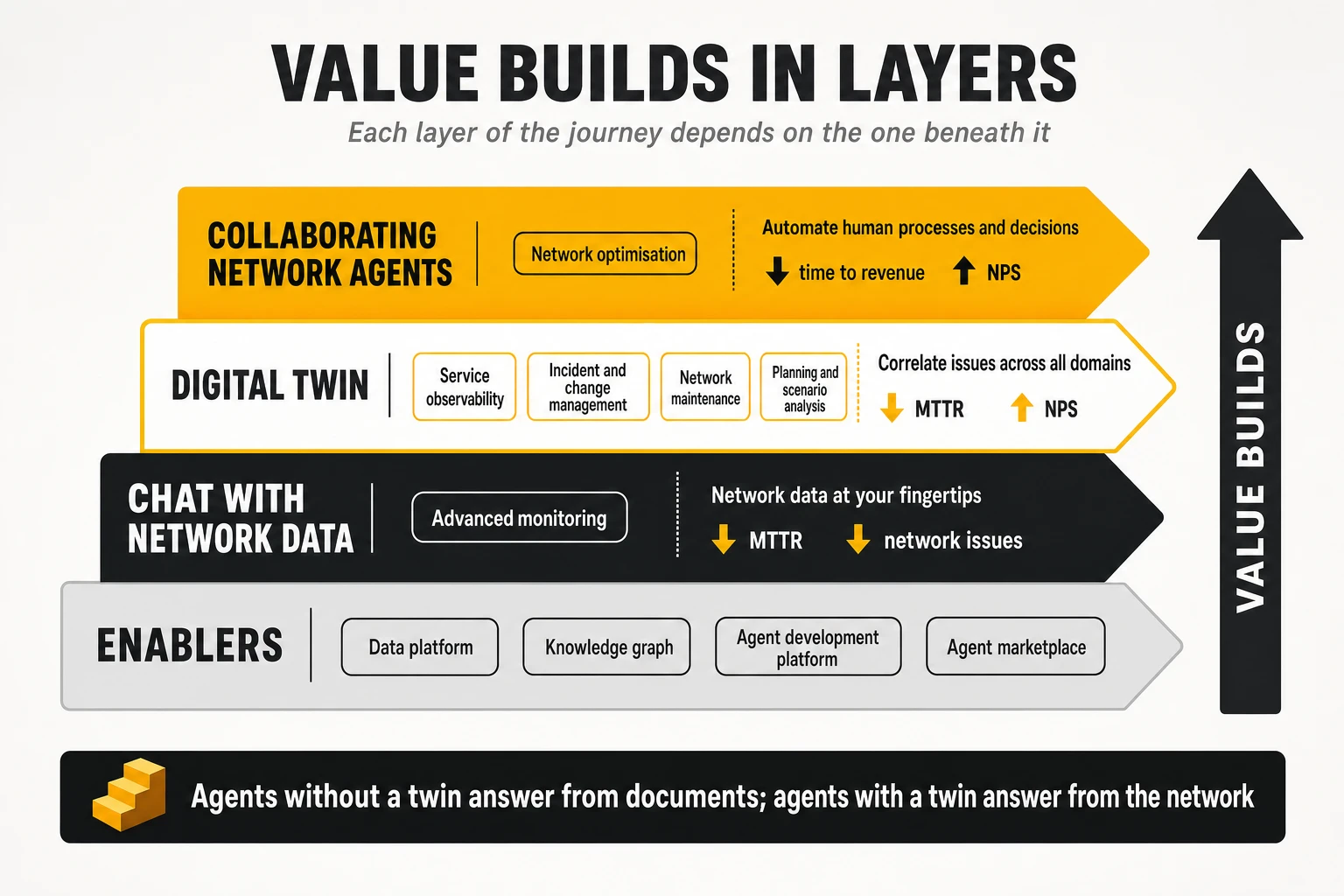
The framework as layers. The digital shadow (Spanner Graph plus BigQuery) is the data core; prediction and agents are built on it; an on-premises gateway handles ingestion, event processing and controlled configuration. Every box can be replaced by a tool the operator already runs. Labels use the framework’s original names: Vertex AI is now Gemini Enterprise Agent Platform, and Agent Engine is now Agent Runtime.

The framework maps onto the model, shadow, twin progression described in section 1. The first phase is a connected inventory in one data source, which allows inventories and configuration databases to be reconciled and the end-to-end topology to be established; the second adds live monitoring to reach a shadow suitable for root cause analysis; the third adds prediction and what-if analysis. Value builds in the same order: enablers first (data platform, knowledge graph, agent platform), then conversational access to network data, then twin-based use cases, and finally collaborating agents.

Value builds in layers: each step depends on the one beneath it. Agents without a twin answer from documents; agents with a twin answer from the network.

Spanner: the database underneath

Spanner is a globally distributed relational database that Google built for its own services. It was described publicly in the 2012 OSDI paper “Spanner: Google’s Globally-Distributed Database” and offered as a Google Cloud service from 2017. It combines SQL, strong consistency and horizontal scaling of both reads and writes, which is an unusual combination: most databases that scale horizontally relax consistency.

For a network twin, three properties matter more than raw scale.

Strong consistency: when an agent reads the topology, it reads a consistent state, not a mixture of before and after an update. Root cause analysis on an inconsistent graph produces confident wrong answers.
Granular sizing: instances start at 100 processing units (a tenth of a node), so a regional pilot does not require a large commitment.
Availability: the Enterprise Plus edition supports multi-region configurations with an availability SLA of up to 99.999%, relevant when the twin becomes part of the incident path.

Edition matters and should be checked early. The graph, full-text search, vector search and columnar engine capabilities require the Enterprise or Enterprise Plus edition; they are not available in Standard.

Spanner Graph: a graph declared over existing tables

The design decision that makes Spanner Graph different from most graph databases is that the graph is declared over relational tables. Generally available since January 2025, it lets the operator keep inventory, alarms and tickets as ordinary tables and then map rows to nodes and edges with a declarative schema — without migrating data or running a separate ETL into a graph store. A minimal network twin schema looks like this:

CREATE PROPERTY GRAPH NetworkTwin
  NODE TABLES (
    Entity KEY (eid),
    Faults KEY (alarm_id),
    Tickets KEY (ticket_id)
  )
  EDGE TABLES (
    EntityToEntity
      SOURCE KEY (eid) REFERENCES Entity (eid)
      DESTINATION KEY (to_eid) REFERENCES Entity (eid)
      LABEL ConnectsTo,
    EntityHasFault
      SOURCE KEY (eid) REFERENCES Entity (eid)
      DESTINATION KEY (alarm_id) REFERENCES Faults (alarm_id)
      LABEL HasFault,
    EntityHasTicket
      SOURCE KEY (eid) REFERENCES Entity (eid)
      DESTINATION KEY (ticket_id) REFERENCES Tickets (ticket_id)
      LABEL HasTicket
  );

The operational consequence is the one that answers the “real time” question every operations team asks. Because nodes and edges are rows, inserting a new router into the Entity table and a new alarm into the Faults table changes the graph in the same transaction. There is no rebuild, no nightly sync and no second copy to drift: two plain SQL INSERT statements, one for the node and one for the alarm, are enough for the next graph query to show both. What remains the operator’s responsibility is the feed: something — an inventory system, a controller, a discovery job — has to write that row.

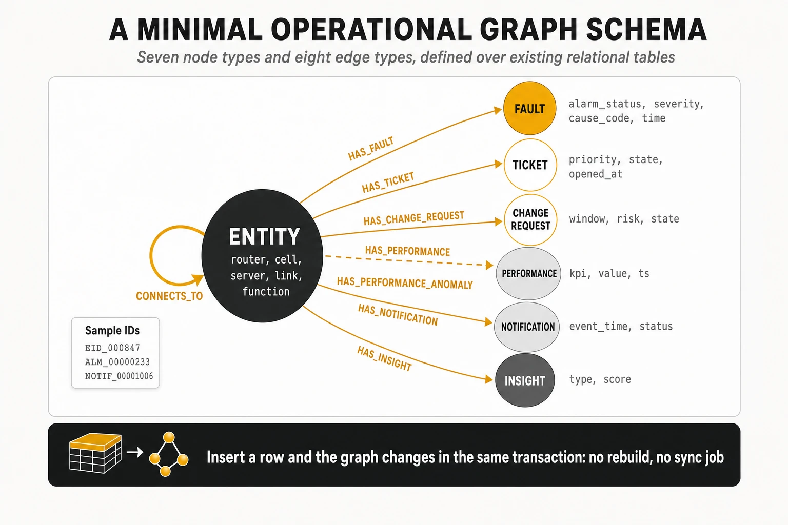
A minimal operational schema: seven node types and eight edge types over existing tables. The entity node carries the network; every other node type carries a kind of state or history attached to it.

Querying the twin with GQL

Queries use the ISO GQL standard, and Spanner’s implementation is based on both GQL and SQL/PGQ, so graph patterns and SQL can be mixed in the same statement. Three examples on the schema above, with illustrative identifiers, show the style.

Neighbours of a given element that have an active fault — the first question in almost every incident:

GRAPH NetworkTwin
MATCH p = (n1:Entity {eid: "EID_000847"})-[:ConnectsTo]->(n2:Entity)
          -[:HasFault]->(f:Faults)
WHERE f.alarm_status = "ACTIVE"
RETURN n2.eid, f.alarm_id, f.alarm_severity, f.cause_code;

The ten radio nodes with the oldest active performance degradation — a query that returns a table, not a picture:

GRAPH NetworkTwin
MATCH (n:Entity)-[:HasFault]->(f:Faults)
WHERE JSON_CONTAINS(n.labels, JSON '{"source_network_segment":"RAN"}')
  AND f.clear_time IS NULL
  AND f.alarm_status = "ACTIVE"
  AND f.cause_code = "PERF_DEGRADATION_CHRONIC"
RETURN n.eid, MIN(f.time) AS fault_start_time
GROUP BY n.eid
ORDER BY fault_start_time ASC
LIMIT 10;

From the worst radio node, every core node within one to four hops that also has an active fault — the blast radius walked upward:

GRAPH NetworkTwin
MATCH (ran:Entity)-[:HasFault]->(f1:Faults)
WHERE f1.cause_code = "PERF_DEGRADATION_CHRONIC" AND f1.clear_time IS NULL
ORDER BY f1.time ASC
LIMIT 1
MATCH p = (ran)-[:ConnectsTo]->{1,4}(core:Entity)-[:HasFault]->(f2:Faults)
WHERE JSON_CONTAINS(core.labels, JSON '{"source_network_segment":"CORE"}')
  AND f2.alarm_status = "ACTIVE"
RETURN TO_JSON(p) AS path
LIMIT 100;

Results can be explored visually. The open-source Spanner Graph Notebook renders query results as interactive graphs in Colab or Jupyter, with a property inspector for each node; the same views are available in the console’s Spanner Studio.

In June 2026 Google added graph algorithms to Spanner Graph, still in preview in October 2026. They are called as built-in functions inside graph queries and run on Data Boost and independent on-demand compute, so they barely touch the provisioned instance; results can be written back to Spanner or exported. The catalogue covers centrality (PageRank, including personalised, betweenness and closeness), clustering (weakly connected components, modularity and correlation clustering, label propagation, clique finding), similarity (Jaccard, cosine, common and total neighbours) and shortest paths. Google’s announcement explicitly lists autonomous network operations and digital twins, for finding vulnerabilities and predicting cascading failures, among the use cases. It is a serious capability rather than an absence; it is also younger and narrower than specialised graph analytics libraries, which section 7 examines.

Text, vectors and graph in one database

The same tables can carry full-text and vector indexes. That allows the hybrid question from section 4 — fibre incidents in the last thirty minutes near a town, on elements within two hops of a service — to run as one statement in one engine, with the ticket free text searched by keyword or by semantic similarity using embeddings. For a network operations centre this removes the separate search cluster and vector store that polyglot designs need, together with the pipelines that keep them in step. Native graph databases now offer the same combination inside the graph engine (section 7), so this is an advantage over polyglot designs rather than over every alternative.

BigQuery: the analytical half, and how data moves between the two

BigQuery holds the history — months or years of KPIs, alarms, tickets and derived features — and the integration between the two stores is native rather than hand-built.

From Spanner to BigQuery: change streams capture every insert, update and delete in near real time and feed BigQuery through Dataflow templates, so history accumulates continuously.
Reading Spanner from BigQuery without copying: federated queries and Spanner external datasets let analysts join live topology with historical data. Both run on Data Boost, separate serverless compute, so heavy analytics do not slow the queries that agents and engineers run on the operational twin.
From BigQuery back to Spanner: reverse ETL exports computed results — risk scores, predicted load, model insights — into Spanner tables, in batch or continuously, where they become node properties or insight nodes. It requires a BigQuery Enterprise or Enterprise Plus reservation.
Catalogue and governance: Google’s data catalogue, renamed Knowledge Catalog in April 2026 (formerly Dataplex Universal Catalog), discovers and documents the data assets on both sides — useful when the first job is to find out what the inventory exports actually contain.

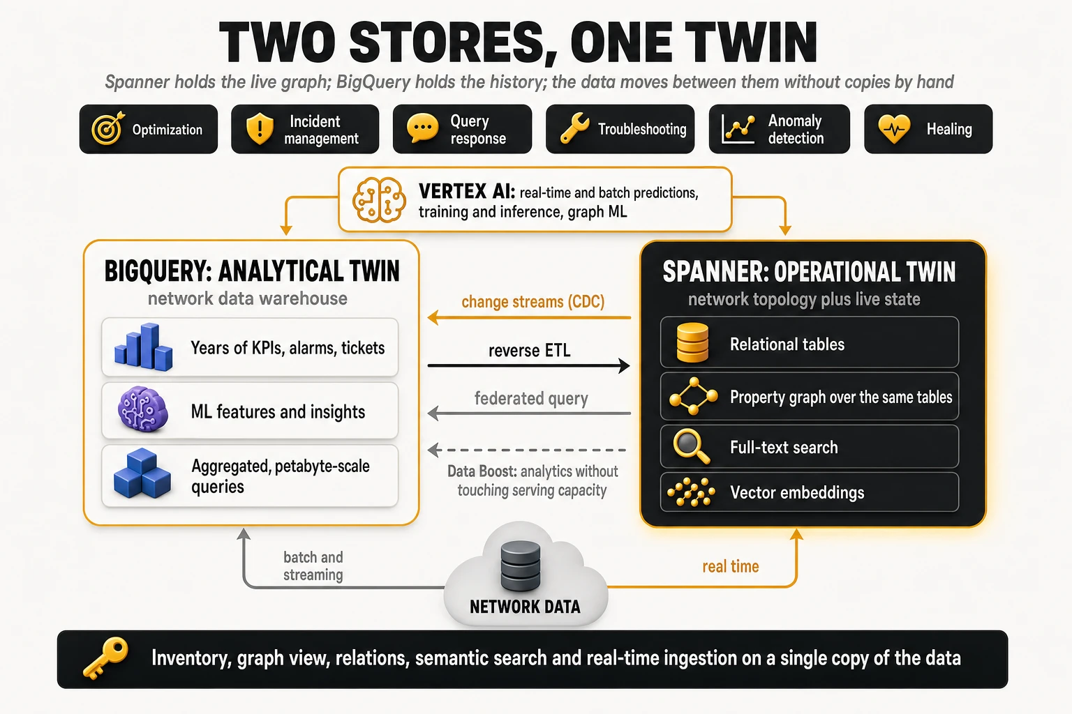
Two stores, one twin: Spanner holds the live graph, BigQuery holds the history, and the data moves between them through native mechanisms rather than hand-written pipelines. The prediction box carries the platform’s former name, Vertex AI.

Vertex AI and graph neural networks

The prediction layer uses Google’s AI platform — Vertex AI, renamed Gemini Enterprise Agent Platform in April 2026 — for training, hosting endpoints and serving predictions in real time or batch. Three model types appear in the framework: forecasting models for traffic and load, generative models for simulation, and graph neural networks for impact and root cause.

A graph neural network (GNN), the fourth layer described in section 2, is a model that learns from the structure of a graph, not only from the values in each row. Each node is represented by an embedding that is updated with information from its neighbours, so the model can learn patterns such as “degradations of this shape on these kinds of elements, connected this way, usually originate two layers below.” Google has used this class of model internally for years and has published the tooling: TensorFlow GNN 1.0 in February 2024 and, in September 2026, Distributed Graph Flow, an open-source library that loads a training graph directly from Spanner Graph and simplifies feature preparation, training and inference for teams without deep graph ML experience.

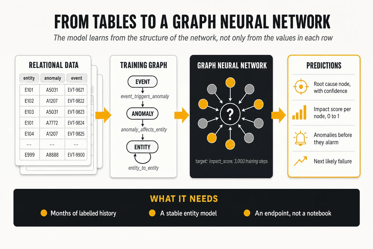
From tables to a graph neural network. The training graph links events, anomalies and entities; the model predicts an impact score per node, from which root cause and ranking follow. It needs months of labelled history and a stable entity model.

The workflow is short to describe and long to do well. Read the graph from Spanner; declare the features of each node set (for example the incident type and root cause of events, the type, criticality and impact score of anomalies, the type, domain and segment of entities); train a node model whose target is a variable such as an impact score from 0 to 1; evaluate; deploy to an endpoint; and call it when a new anomaly is written to the graph. Training takes hours, inference milliseconds. Algorithm-discovery agents such as Google DeepMind’s AlphaEvolve are a research direction for the optimisation problems of the full-twin level, not an operational component today.

Agents: from tools to an operator interface

The agent layer is built with Google’s Agent Development Kit (ADK), runs on the platform’s agent runtime and is exposed to engineers through Gemini Enterprise, launched in October 2025. Agents reach the twin through tools defined with the MCP Toolbox for Databases, which exposes Spanner through the Model Context Protocol; agents from different suppliers coordinate through the Agent2Agent (A2A) protocol, now hosted by the Linux Foundation.

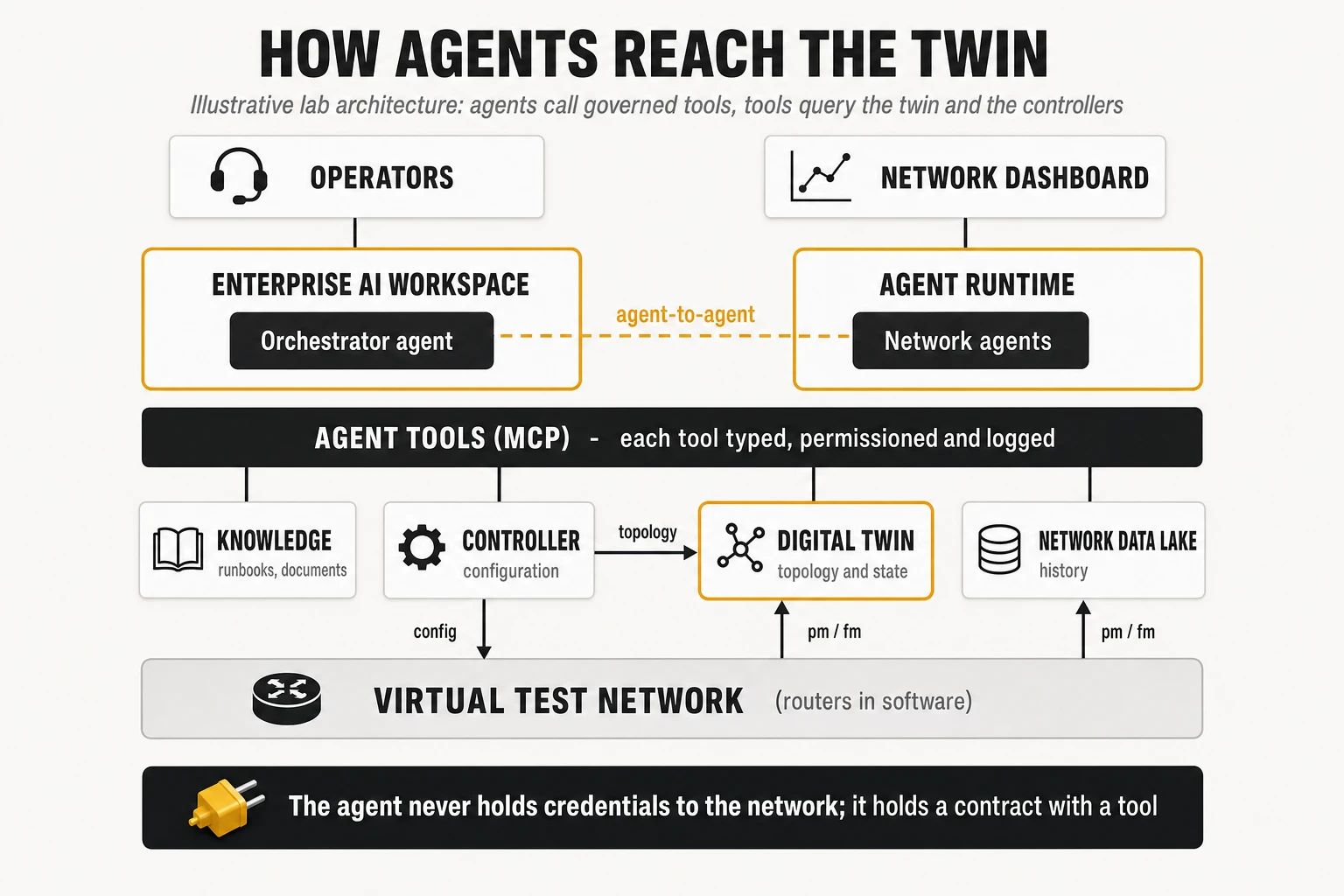
How agents reach the twin, in an illustrative test architecture. Agents call typed, permissioned tools; the tools query the twin, the knowledge base and the controllers. The agent never holds credentials to the network.

Consider how a conversational network agent works on even a small graph. An engineer asks which switches are in a critical state; the agent queries the twin and lists them. The engineer asks what one of them is connected to; the agent returns the neighbourhood as a graph. “Expand to two hops” produces a denser topology; “show me the paths between these two faulty nodes” returns every path; “only the shortest” returns one path through a specific tower. Each question becomes a graph query issued by a tool, which is why the answers can be audited — and why an agent without the twin would only be able to answer from documents.

What is strong, and what to check before committing

Strengths, in TelcoCrux’s assessment.

SQL and graph on the same rows: when the operational data is already relational, the graph needs no second copy, and the “real time” claim is concrete — the graph is as current as the last committed row. This does not remove the pipelines from inventory and OSS into those tables, and a native graph database has no internal copy to synchronise either; the advantage is specific to data that lives, or should live, in relational form.
One operational engine for relational, graph, text and vector simplifies hybrid queries that network operations actually need, without a separate relational store.
Distributed scale and global consistency: horizontal write scaling and strongly consistent reads across regions are native to the service.
The analytical integration is native: change streams, federated queries, Data Boost and reverse ETL cover the loop between live and historical data without custom pipelines.
The path from twin to graph ML is short, with an open-source library that reads the twin directly.
The framework is modular; an operator can adopt the twin without adopting the agent stack, or vice versa.

Points to verify, because they decide cost and risk.

Editions and reservations: graph, search and vector features need Spanner Enterprise or higher; reverse ETL needs a BigQuery Enterprise reservation. Price the pilot and the production estate with those editions, not with list prices for the basic tier.
Data residency and sovereignty: topology and customer mappings are sensitive. Check region availability, encryption key control and any sovereign-cloud requirement before the first export leaves the building.
The on-premises gateway: ingestion, event processing and any configuration path into the network remain the operator’s integration work.
Graph engine maturity for the operator’s queries: test the heaviest traversals — deep variable-length paths across the full estate — at production scale, not on a regional sample. Graph algorithms were still in preview in October 2026, and their breadth is narrower than that of specialised graph analytics libraries.
Deployment model: Spanner is a Google Cloud service. An operator whose policy requires topology data to stay in its own data centres cannot run it on premises.
Name churn: several components were renamed in 2026 (the AI platform, the agent runtime, the catalogue). That is cosmetic, but contracts and architecture documents should reference capabilities, not product names.
Public operational evidence: Google’s published operator examples — including a 2026 proof of concept with a Spanner Graph twin holding billions of dependencies and a fine-tuned GNN for root cause — describe architectures and intent more than measured before-and-after results. Ask for measured outcomes on comparable estates.

7. Neo4j: from the operational graph to graph data science and agents

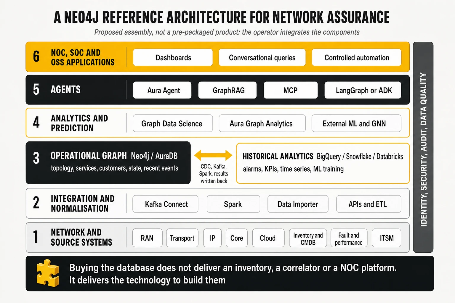
Neo4j starts from the opposite end of the problem. Google builds the twin as part of an integrated cloud data and AI platform, with the graph declared over a distributed relational database. Neo4j starts from a database whose only job is to store and traverse relationships, and extends it outwards: a large library of graph algorithms, on-demand analytics sessions, graph-grounded generative AI, agent tooling, and connectors to whichever warehouse and streaming platform the operator already runs.

That makes the comparison a two-level one, and it is unfair to compare only one level. At the database level, Spanner Graph is compared with Neo4j’s database (self-managed, or AuraDB as a managed service). At the solution level, Spanner plus BigQuery plus Google’s AI and agent platform is compared with Neo4j plus Graph Data Science plus the operator’s warehouse plus GraphRAG and agent tooling. Section 6 described Google at the solution level; this section does the same for Neo4j.

Level	Google Cloud	Neo4j
Operational database	Spanner with Spanner Graph	Neo4j Database (self-managed) or AuraDB (managed)
Full solution	Spanner, BigQuery, Gemini Enterprise Agent Platform, ADK agents	Neo4j, Graph Data Science or Aura Graph Analytics, the operator’s warehouse, GraphRAG, Aura Agent or MCP-based agents
Architectural priority	Integration of data models and distributed scale	Specialisation in relationships and graph analytics

The two levels of the comparison. Comparing Google’s full solution with Neo4j’s database alone would understate Neo4j; comparing Neo4j’s full ecosystem with Spanner alone would understate Google.

There is one distinction to keep in mind throughout. Buying Neo4j does not deliver a network inventory, an alarm correlator or a NOC platform. It delivers the technology to build a large part of them — as does buying Spanner. The reference architecture below is a TelcoCrux proposal for network assurance, not a pre-configured Neo4j product.

A Neo4j reference architecture for network assurance: the operational graph in Neo4j or AuraDB, history in the operator’s warehouse, Graph Data Science for structural analytics and an agent layer on top. A proposed assembly, not a packaged product.

The database: a native property graph

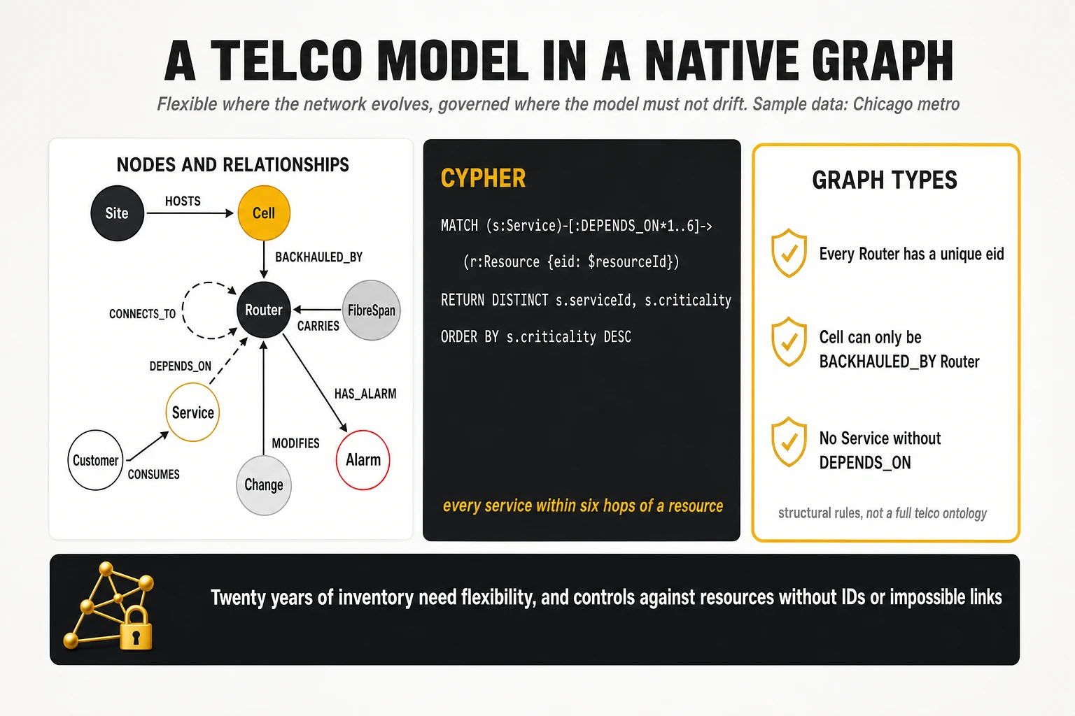
Neo4j is a native property graph database: nodes and relationships are the storage itself, not a view over tables. A relationship is a stored record that points directly from one node to another, so a traversal follows those pointers rather than computing joins. For infrastructure in which dependencies and paths are the core of the model, that is a natural fit. The telco model from section 2 is written directly as entities and connections, without first designing tables and then declaring a graph over them.

Node labels	Relationship types	Example
Site, Cell	HOSTS	Site CHI-0311 hosts cell CHI-0311-B2
Cell, Router	BACKHAULED_BY	The cell is backhauled by aggregation router AGG-CHI-114
Router, Router	CONNECTS_TO	Aggregation router to core router
FibreSpan, Router	CARRIES	Span CHI-SPAN-07 carries the uplink
Service, Resource	DEPENDS_ON	Enterprise VPN 77810 depends on the router
Customer, Service	CONSUMES	A hospital group consumes the VPN
Router, Alarm	HAS_ALARM	The router has active alarm ALM-9182
Change, Router	MODIFIES	A change request modifies the router

A minimal telco model in a native graph, with illustrative Chicago-area identifiers. The same entities as in the Spanner example of section 6, expressed directly as nodes and relationships.

The same telco model as a native graph. Cypher expresses variable-depth dependency questions compactly; graph types add structural rules where the model must not drift.

Cypher, Cypher 25 and the GQL standard

Neo4j’s query language is Cypher, the declarative graph language that strongly influenced the ISO GQL standard. Since Neo4j 2025.06 there are two versions: Cypher 5, now frozen except for fixes, and Cypher 25, which receives all new features and is the default for new databases from 2026.02. Neo4j publishes its GQL conformance in detail: Cypher 25 supports most mandatory GQL features and a good share of the optional ones, but it is not fully conformant. Neither is Spanner’s dialect, so queries are similar in style and not automatically portable between the two engines.

A variable-depth dependency question is short to express. Every service that depends, directly or through up to six intermediate elements of any type, on a given resource:

MATCH (s:Service)-[:DEPENDS_ON*1..6]->(r:Resource {eid: $resourceId})
RETURN DISTINCT s.serviceId, s.criticality
ORDER BY s.criticality DESC;

The neighbours of an element that carry an active major alarm — the first question in an incident, as in section 6:

MATCH (r:Router {eid: "AGG-CHI-114"})-[:CONNECTS_TO]-(n)-[:HAS_ALARM]->(a:Alarm)
WHERE a.status = "ACTIVE" AND a.severity IN ["MAJOR", "CRITICAL"]
RETURN n.eid, a.alarmId, a.severity, a.cause;

Is Neo4j faster than Spanner Graph for these queries? It cannot be stated in general. Neo4j is built for traversal and has extensive optimisations for patterns and paths; Spanner brings distributed execution. Real performance depends on cardinality, depth, selectivity, data distribution, indexes and concurrency. The only honest answer is to run the same questions on a comparable topology, which is what the benchmark in section 13 is designed to do.

Modelling and governance: flexible where it must be, strict where it matters

Neo4j has traditionally used a flexible schema: new node labels and relationship types can be added as new domains or source systems appear, without a migration. For a model that has to absorb twenty years of inventory conventions, that flexibility is valuable during discovery and dangerous in production, where it allows resources without identifiers, impossible relationships and duplicated inventory to creep in.

Graph types, generally available since Neo4j 2026.06, close much of that gap. Graph types (Cypher 25 only; Enterprise Edition, Infinigraph and Aura) let the operator declare structural rules for the node labels and relationship types it names — which properties are mandatory, which are keys, which relationship types may connect which labels — while leaving the rest of the graph open. Existing constraints are folded into the graph type automatically. A classic key constraint looks like this:

CREATE CONSTRAINT router_eid IF NOT EXISTS
FOR (r:Router) REQUIRE r.eid IS NODE KEY;

Graph types are structural rules, not a telco ontology. They will stop a cell from being backhauled by a customer; they will not decide what “in service” means in each inventory. The TelcoCrux assessment is that Neo4j combines flexible modelling well with governance over the stable parts of the graph; Spanner offers rigour through a more relational, declarative approach in which the tables define the structure from the start.

Keeping the graph current: Kafka, CDC and transactions

A point that is easy to misread in comparisons: Neo4j does not need to synchronise two stores to keep its operational graph current. Nodes and relationships live in one database and change inside ACID transactions (atomic, consistent, isolated and durable); when an event updates a router node, the new state is visible to every query once the transaction commits. That is the same property Spanner offers, reached through a different storage model.

The real work, on either platform, is turning a source event into the right change in the graph. Take an alarm emitted by a fault management system:

{
  "resource": "RTR-CHI-0042",
  "alarm_id": "ALM-9182",
  "severity": "CRITICAL",
  "status": "ACTIVE"
}

In Neo4j, an integration maps that event to an update of the router node and its relationship to an alarm node. The official Neo4j Connector for Kafka works in both directions: as a sink it consumes Kafka topics and writes to Neo4j or AuraDB with a mapping such as the one below; as a source it publishes changes from the graph to Kafka, using change data capture or a polling query. It is available for Confluent Platform and Cloud and for open-source Apache Kafka, including Amazon MSK.

MERGE (r:Router {eid: $event.resource})
MERGE (a:Alarm {alarmId: $event.alarm_id})
SET a.severity = $event.severity, a.status = $event.status, a.raisedAt = datetime()
MERGE (r)-[:HAS_ALARM]->(a);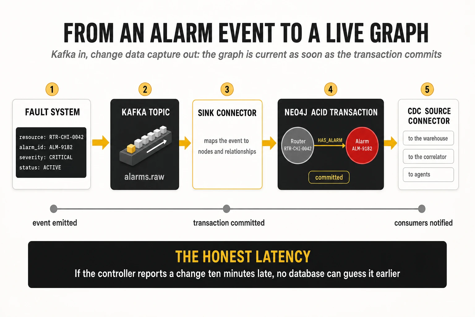

From an alarm event to a live graph and back out. The graph is current once the transaction commits; CDC publishes the change to every consumer. Identifiers are illustrative.

Change data capture has edition requirements that matter for budgeting. CDC is available in Enterprise Edition and in AuraDB Business Critical and Virtual Dedicated Cloud, not in the Professional tier. The comparison with Google, function by function:

Aspect	Spanner Graph	Neo4j
Graph update	Transaction on the underlying tables	Transaction on nodes and relationships
When the change is visible	After commit	After commit
External feeds	Pipelines, APIs, Dataflow, connectors	Kafka connector, APIs, Spark, connectors
Change data capture to consumers	Spanner change streams	Neo4j CDC plus the Kafka source connector
Main integration effort	Mapping sources to tables, data quality	Mapping sources to nodes and relationships, data quality

A functional tie on keeping the graph current, with different architectures. On both, real freshness depends on the source systems and the ingestion chain: if a controller reports a change ten minutes late, no database can know it earlier.

Graph Data Science: Neo4j’s strongest argument

Graph Data Science (GDS) is the part of Neo4j that most distinguishes it for network work. It is a library of algorithms that run on in-memory projections of the graph and compute properties of the structure itself — not answers to a specific question, but facts such as which nodes many paths depend on, which links hold the network together and which groups of elements behave as a cluster. Algorithms are classified by maturity tier, and the reference list shows which are production-ready.

Algorithm or technique	What it finds	Network application	GDS tier
Betweenness centrality	Nodes that many shortest paths cross	Routers whose failure would reroute most traffic	Production
Articulation points	Nodes whose removal disconnects the graph	Single points of failure	Production
Bridges	Links whose removal breaks connectivity	Critical transport links	Production
Dijkstra and weighted shortest paths	Minimum-cost paths	Routes by latency or modelled cost; reroute options	Production
Louvain and Leiden community detection	Tightly connected groups	Infrastructure clusters and dependency domains	Production
PageRank	Structural importance	Prioritising resources for protection or audit	Production
FastRP node embeddings	Structure encoded as vectors	Finding topologically similar sites or failure contexts	Production
GraphSAGE embeddings	Learned, inductive embeddings	Generalising to new nodes	Beta
Link prediction pipelines	Relationships likely to exist	Candidate missing links in the inventory	Beta

Graph algorithms that matter to a network, with their maturity tier in the GDS reference as of the 2026.09 release. Several of the most useful ones for assurance are production-grade.

Graph algorithms that matter to a network. They are deterministic mathematics on the topology and need no neural network; their maturity varies by algorithm.

A worked example shows why this matters economically. Imagine 50,000 routers and switches in a Midwest metro and regional network, with hundreds of thousands of links carrying enterprise services. A conventional correlation engine detects that a link is down and looks up what depends on it. Graph Data Science goes further, before anything fails:

Compute articulation points and bridges: the nodes and links whose loss would split the network.
Compute betweenness centrality and PageRank for every router: structural importance.
Cross those results with redundancy, commercial criticality and utilisation from the inventory and the warehouse.
Produce a ranked list of preventive interventions and change scenarios.

CALL gds.graph.project('transport', 'Router',
  {CONNECTS_TO: {orientation: 'UNDIRECTED'}});

CALL gds.articulationPoints.stream('transport')
YIELD nodeId
RETURN gds.util.asNode(nodeId).eid AS singlePointOfFailure;

CALL gds.betweenness.write('transport', {writeProperty: 'betweenness'});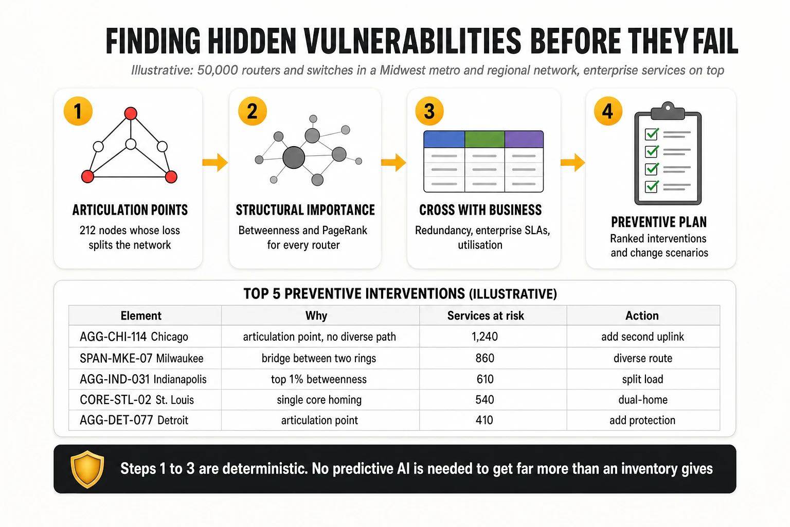

Finding hidden vulnerabilities before they fail. Steps 1 to 3 are deterministic; no predictive AI is needed to learn far more than the inventory shows. Elements and figures are illustrative.

The first three steps need no learned model. That is the economic point: a large gain in network intelligence over a conventional inventory comes from deterministic mathematics that is explainable, reproducible and cheap to run. It also fills the middle ground between rules and machine learning described in section 3.

Graph algorithms are not graph neural networks

This is the boundary between layers 3 and 4 of section 2. GDS provides graph algorithms, embeddings and some machine learning pipelines; a graph neural network is a family of deep learning models that learn by exchanging information between nodes and their neighbours. GDS includes GraphSAGE, an inductive embedding method, in beta, and the graph can be exported to external frameworks such as PyTorch Geometric for deeper models. So Neo4j does not amount to a complete platform for training and serving deep GNNs — and neither does Google’s database by itself: Distributed Graph Flow makes the process easier, but modelling, training and validation remain work to do on both.

Aura Graph Analytics: heavy compute away from the live graph

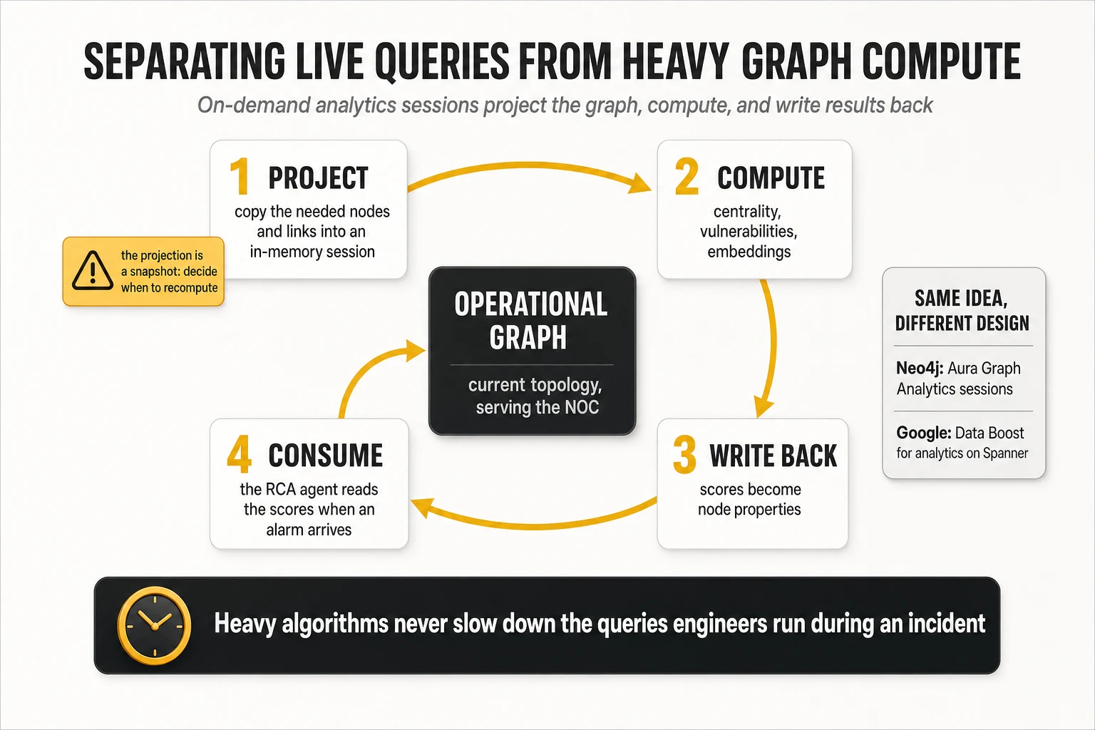
Running algorithms over a whole national topology is heavy, and it must not slow down the queries engineers run during an incident. Neo4j’s answer is Aura Graph Analytics, launched in May 2025: serverless, pay-as-you-go sessions that run GDS workloads in isolated compute. A session projects the data it needs, runs algorithms or models, and writes the results back. Sources can be AuraDB, self-managed Neo4j (through a private link) or non-Neo4j data loaded as data frames; the published price is $0.40 per GB of session memory per hour.

Separating live queries from heavy graph compute. Neo4j uses on-demand analytics sessions; Google uses Data Boost on Spanner. Same idea, different design.

In practice the pattern is simple. The operational graph keeps the current topology; a session computes centrality, vulnerabilities or embeddings overnight or after significant changes; the results are written as node properties; a root cause agent reads them when an alarm arrives. The limitation is equally simple: the projection is an in-memory snapshot and is not synchronised with every new transaction, so the operator must decide when to recompute. Google’s equivalent on the database side is Data Boost, which also runs Spanner Graph algorithms on independent compute; on the analytics side BigQuery is built for very large tabular history and aggregation, while graph analytics sessions are built for computation over structure. They are not substitutes for each other.

History: Neo4j with BigQuery, Snowflake or Databricks

Neo4j follows the same two-store principle as Google, but through connectors rather than one managed ecosystem. The Neo4j Connector for Apache Spark moves data in both directions between Neo4j and Spark, with documented use on Databricks and data warehouses including Snowflake, BigQuery, Redshift and Synapse; the Kafka connector and CDC carry continuous changes. The integration between Spanner and BigQuery is more tightly coupled and managed inside one ecosystem; Neo4j requires more integration decisions and, in exchange, leaves the operator free to keep the warehouse it already has.

The design rule is the same on both platforms. Millions of historical samples of every KPI do not belong in the operational graph. The graph holds the network entities, their relationships, the relevant current state, recent events and analytical summaries; the warehouse or a time-series platform holds the bulk history.

A temporal property is not a temporal graph. Neo4j stores dates and times on nodes and relationships, but reconstructing what the topology looked like last Tuesday — which root cause analysis, change analysis and decision audits need — requires an explicit versioning design for nodes and relationships. Spanner does not solve the historical meaning of business relationships by itself either. Whichever engine is chosen, temporal modelling is a design task to plan from the start.

Generative AI and agents: Neo4j’s own offer

Neo4j has built a substantial generative AI layer around the graph. Its native vector indexes (generally available since Neo4j 5.13) and full-text indexes sit inside the graph database, and since 2026 a single SEARCH clause covers both. On top, the official GraphRAG library for Python combines vector search, full-text search, hybrid retrieval, graph traversal to expand context, and translation of natural language into Cypher.

Consider a question a NOC engineer actually asks: “Which enterprise services depend on the affected router, and which of them had similar incidents in recent weeks?” An agent runs a structural traversal from the router to services and customers, a semantic search over ticket text for similar incidents, and a keyword search for specific terms, then asks a language model to synthesise an answer that cites the nodes and tickets it used. The graph supplies the structure of dependencies; the model supplies the interaction and the synthesis.

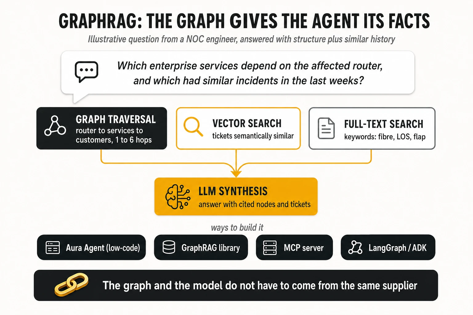
GraphRAG: the graph gives the agent its facts. The graph and the language model do not have to come from the same supplier.

There are three ways to put this in front of engineers.

Aura Agent, generally available since February 2026, is a low-code platform inside AuraDB for building agents grounded in a knowledge graph. It can draft an agent from the graph schema and a description of the use case, and deploy it as a REST API or as an OAuth-secured, cloud-hosted MCP endpoint.
The official Neo4j MCP server exposes the schema, read and write Cypher and Graph Data Science algorithms to any agent framework that speaks the Model Context Protocol. Separate Neo4j Labs servers cover data modelling and other tasks, without product support.
External frameworks such as LangGraph or Google’s Agent Development Kit can use those MCP tools, with permissions and restrictions set by the operator.

The consequence is that an operator can build agents with Gemini and ADK that query Neo4j as their operational knowledge base. Nothing obliges the graph and the language model to come from the same supplier. What Aura Agent does not replace is a full orchestration platform for autonomous operations: a closed loop that involves controllers, ITSM, verification, policies and other agents still needs a broader execution architecture, which the operator builds or buys.

Scale, consistency and deployment

Distributed scale was historically the clearest argument for Spanner, and in 2026 the comparison has moved, though not closed. Neo4j scales through clustering: primaries replicate writes with the Raft protocol, so a commit needs a majority of primaries; secondaries are asynchronous read replicas that scale reads. Composite databases query several graphs as one, although a transaction can write to only one of them. And since December 2025 Infinigraph adds property sharding: the graph structure stays in one replicated shard while properties are spread across property shards, which matters for very large graphs with heavy properties. Infinigraph needs a specific subscription and is not available on Aura, and it is not the same as transparently distributing every write of an arbitrary graph.

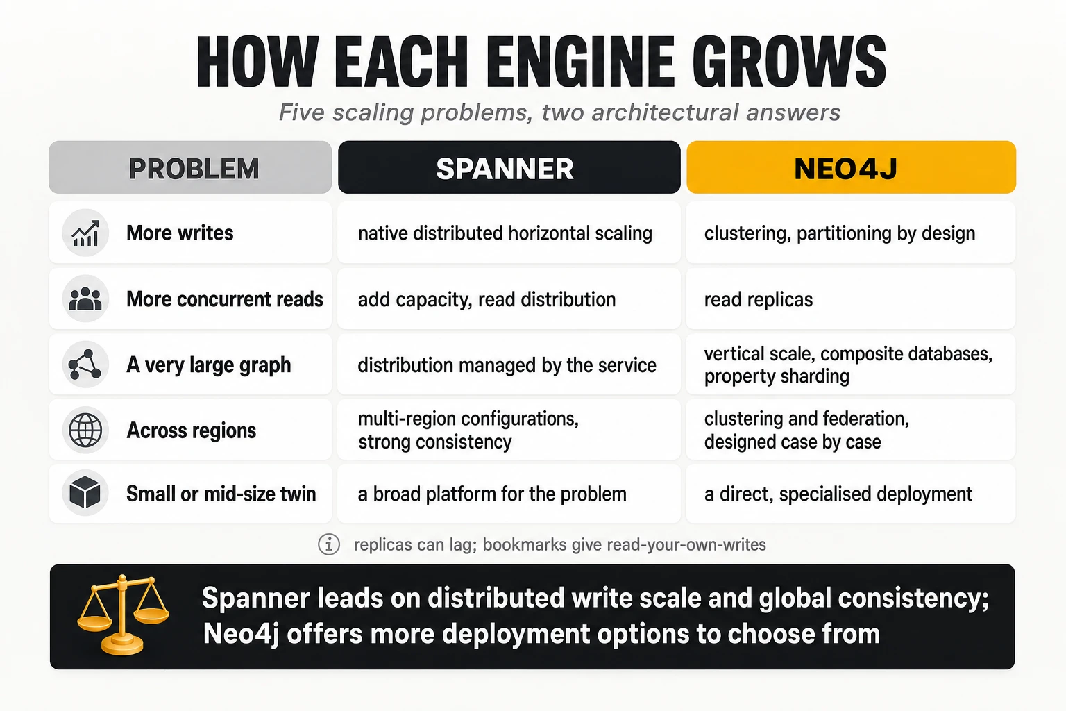
How each engine grows. Spanner leads on distributed write scale and global consistency; Neo4j offers more deployment options to choose from.

Consistency deserves precision. Neo4j is ACID, but in a cluster the secondaries can lag behind; causal consistency through bookmarks guarantees that a session reads its own writes. Spanner offers strongly consistent reads with global guarantees in the corresponding configurations. For a twin that agents read during an incident, both models work if they are used correctly; they are not the same guarantee.

Deployment flexibility is where Neo4j leads clearly. AuraDB runs on AWS, Azure and Google Cloud, including through the Google Cloud Marketplace; Enterprise and Infinigraph editions can be self-managed on premises or in any cloud. An operator whose policy requires topology and customer mappings to stay in its own data centres can run Neo4j there; it cannot run Spanner there.

Exploration and the people who use the graph

Neo4j’s visual exploration tool, Bloom, lets engineers who do not write queries search, expand neighbourhoods, find shortest paths and export views. This is not cosmetic. A twin that only data engineers can interrogate stays a data project; one that a transport planner or a NOC shift lead can explore becomes part of the operation. Google offers the open-source Spanner Graph Notebook, Spanner Studio and third-party visualisation partners; the TelcoCrux assessment is that Neo4j’s tooling for interactive exploration is more mature.

Public evidence in telecom

Neo4j has the longer list of public telecom references, with one that includes measured results.

BT Group: its Service and Resource Inventory Management System (SRIMS) consolidates hundreds of inventory systems into a digital twin of its wholesale network inventory, replacing an earlier graph system. BT and Neo4j report 60% fewer human decision points, 50% less time spent on capacity planning and around 3,000 users. These are published customer-story figures, not an independent audit, and the story gives no project date.
Comcast: presented in September 2025 a graph-powered digital twin of its nationwide network that connects every network layer, used to trace equipment and help resolve incidents. The public presentation gives no comparable figures for latency, root cause precision or MTTR.
Sopra Steria: its Intelligent Network Analyzer is a what-if and fault analysis tool for mobile networks built on Neo4j, used with an operator that is not named.

What is strong, and what to check before committing

Strengths, in TelcoCrux’s assessment.

Specialisation in relationships: a native graph engine with a mature query language, built for exactly the dependency and path questions a twin exists to answer.
Graph Data Science: the broadest and most mature set of graph algorithms in the comparison, with the most useful ones for assurance — articulation points, bridges, centrality, shortest paths, communities — at production tier.
Deployment freedom: managed on three clouds, or self-managed on premises; a decisive factor for operators with sovereignty requirements.
Choice of surrounding stack: any warehouse, any streaming platform, any agent framework through MCP.
Exploration and adoption: visual tools that let non-specialists use the graph.
Telecom references, including one with published operational metrics.

Points to verify.

Editions and features: CDC needs Enterprise or AuraDB Business Critical and above; Infinigraph needs its own subscription and is not on Aura; graph types need Cypher 25. Map every feature in the design to the edition that provides it.
Integration effort: history, streaming and orchestration are assembled, not bundled. Budget the engineering to build and operate the pipelines, the analytics projections and their refresh policy.
Scale at national size: test the largest graph and the heaviest write load on the deployment model actually contemplated, including the behaviour of read replicas under incident load.
Temporal modelling: design the versioning of topology before the first load, not after the first audit.
Cost model: AuraDB is priced per GB of memory per hour — $0.09 for Professional and $0.20 for Business Critical, with a 2 GB minimum and a 99.95% SLA on the latter — and analytics sessions are priced separately. Graph size in memory drives the bill.

8. Building the twin from CSV files: the step that changes the economics

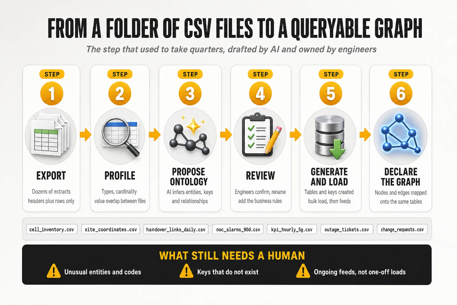
For most operators, the obstacle to a network twin was never the database. It was the model: deciding what the entities are, which columns are keys, which files relate to which, and writing the loading logic for dozens of sources. Historically that work took quarters of interviews, spreadsheets and data engineering before the first useful query. It is also the step where generative AI now makes the largest measurable difference, because the input to it — a folder of exports — is exactly the kind of semi-structured material large language models handle well.

From a folder of CSV files to a queryable graph. The ontology is drafted by AI from headers and contents and owned by engineers; unusual entities, missing keys and ongoing feeds still need people.

The six steps

The route starts from the least structured input possible: dozens of CSV extracts with nothing but a header row and data. No data dictionary, no entity-relationship diagram, often no consistent naming across files.

Export. The operator extracts inventory, topology, alarm history, performance KPIs, tickets and change records for one domain and one region, as flat files. For a radio-focused pilot that can mean thirty to sixty files: cell inventory, site coordinates, antenna sector configuration, physical topology, handover links between cells, daily and hourly KPIs per technology, availability and energy-saving counters, outage history, outage tickets and alarm exports from the fault manager.
Profile. Each file is profiled automatically: column types, cardinality, null rates, value distributions and — critically — value overlap between columns of different files. A column called cell_name in one file and CELL_ID_EXT in another that share 97% of their values are probably the same key.
Propose the ontology. A large language model receives the headers, the profiles and samples of the rows, and proposes entities, primary keys, foreign keys and relationships: which files describe things (nodes), which describe links between things (edges) and which describe states over time (properties or event nodes). In Google’s architecture this is the “ontology tool” built on Gemini, a component of the solution rather than a feature of the database; on Neo4j the same step is an LLM prompted with the profiles and sample rows, run by the operator or its integrator.
Review. Domain engineers confirm, rename and correct. They add what the data cannot reveal: business rules, the meaning of internal codes, which status values mean “in service”, which relationships are physical and which administrative.
Generate and load. On Spanner, the reviewed model becomes table definitions and keys and the files are bulk-loaded. On Neo4j, it becomes node labels, relationship types and constraints, loaded with the visual Data Importer for CSV files, with Spark for large volumes, or with Cypher bulk loads. In both cases the same mapping is reused to build the recurring feeds.
Declare and validate the graph. On Spanner, node and edge tables are mapped onto the loaded tables with the property graph statement shown in section 6; on Neo4j, the graph already exists once the load completes, and graph types or constraints lock down its structure. Then a set of validation queries checks that known facts — a site’s cells, a ring’s members, a known outage’s affected elements — come back correctly.

The same route on each platform

The six steps are identical on both platforms; the tools differ, and neither database infers a telco ontology by itself. Neo4j’s Data Importer makes the modelling and mapping of CSV files visual and quick, and its GraphRAG library includes an experimental knowledge graph builder that extracts entities and relationships from unstructured text with a language model. Extracting a graph from documents, however, is not the same as reconciling thirty inventory files with contradictory keys. On Google’s side, the Gemini-based ontology assistant is part of the solution assembled around Spanner, not an automatic function of the database. On both, steps 2 to 4 are where the operator’s engineers and an LLM do the real work.

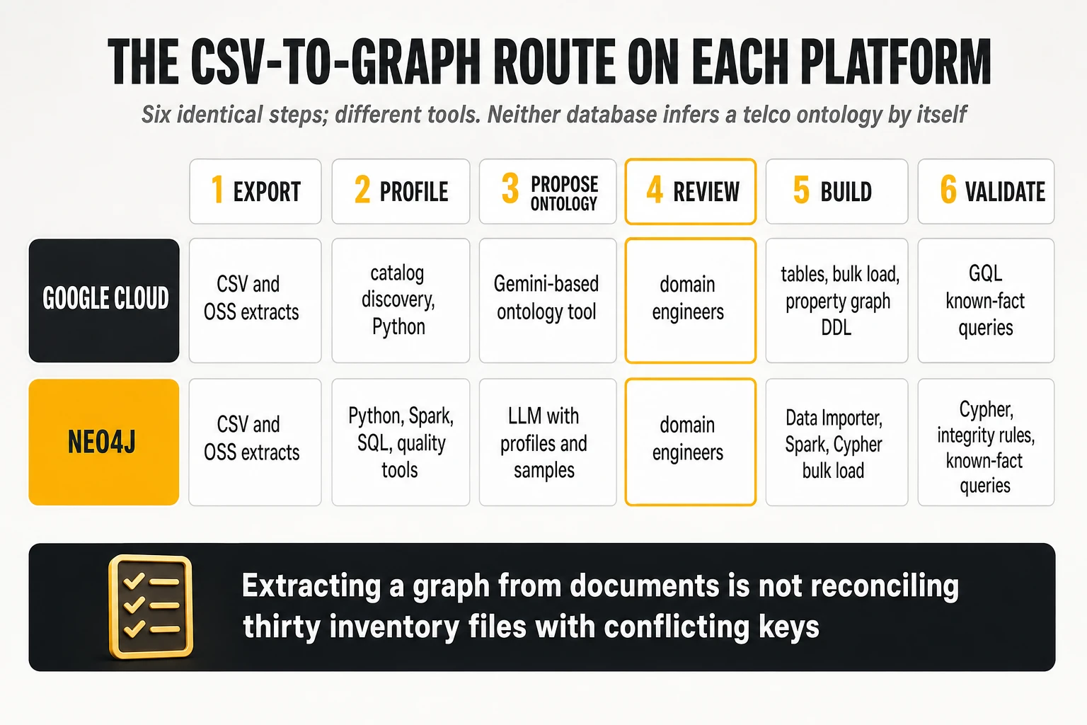
The CSV-to-graph route on each platform: identical steps, different tools. The review step is the same on both, and it is human.

Step	Google Cloud implementation	Neo4j implementation
1. Export	CSV and OSS extracts	CSV and OSS extracts
2. Profile	Catalogue discovery, Python, SQL	Python, Spark, SQL, data quality tools
3. Propose ontology	Gemini-based ontology tool with profiles and samples	LLM with profiles and samples
4. Review	Domain engineers and data owners	Domain engineers and data owners
5. Build	Tables and keys, bulk load, property graph DDL	Data Importer, Spark, Cypher bulk loads, constraints and graph types
6. Validate	GQL queries on known facts	Cypher queries on known facts and integrity rules

The same six steps on each platform. The process is viable and largely automatable on both; on neither is ontology discovery from inventory CSV files a finished, out-of-the-box product feature.

An illustrative regional dataset

A realistic radio-focused pilot for one US region produces a table set like this. Names are illustrative; the structure mirrors what operators typically hold.

Group	Example tables	Becomes in the graph
Inventory and location	CellInventory, SiteCoordinates, AntennaSectorConfiguration, CellRadioConfiguration	Site, cell and sector nodes with location, band, azimuth and configuration properties
Topology	CellPhysicalTopology, BackhaulLinks, TransportRingMembership	CONNECTS_TO, BACKHAULED_BY and RIDES_ON edges
Mobility	CellHandoverLinks, NeighborHandover4G4GDaily, NeighborHandover5G5GDaily, NeighborHandover5G4GDaily	Handover edges between cells, weighted by attempts and success rate
Performance	4G and 5G daily and hourly KPI tables, availability and power-saving counters, energy per network element	Time-stamped performance nodes or properties attached to cells
Faults and outages	Fault manager alarm exports, CellOutageHistory, CellOutageTicketCheck	Fault and outage nodes with HAS_FAULT edges, linked to tickets
Experience	HTTP and bandwidth measurements, enriched measurements from drive tests or apps	Quality-of-experience evidence attached to cells and corridors

A regional radio dataset as a twin. In a pilot of this kind the tables total a few gigabytes, which is small for the database and large enough to answer real operational questions.

What really changes, and what does not

The acceleration is real and should be stated precisely. Run this way, a first usable model can be produced from raw CSV files in a matter of weeks, with a few working sessions with the operator’s engineers to confirm entities and keys, where a hand-built ontology typically took months. The model is a draft, but a draft good enough to load and query is the point at which domain experts become productive, because they can correct an answer instead of designing a schema.

Three things do not change, and the sceptics are right to insist on them.

Everything must be reviewed. Models infer common entities well — locations, identifiers, dates — and are less reliable with unusual ones: proprietary codes, overloaded fields, entities that exist only in one team’s conventions. AI is a large help in drafting the model, and every part of the draft still has to be checked by people who know the network.
Some keys do not exist. When a source exposes a handful of fields and none of them identifies the element unambiguously, no model can infer the join; someone must create the key, usually upstream.
A one-off load is not a twin. The CSV route builds the model and the first state. The shadow requires feeds — events from inventory, controllers and fault management — and those are integration projects with the operator’s systems. The CSV step shortens the time to the first answer; it does not remove the integration.

The practical conclusion is to use the CSV route for what it is good at: proving value on a bounded domain quickly, before committing to integration. If the first twenty questions from the operations centre are not answered better than today, no amount of integration will fix that.

9. Spanner Graph versus Neo4j, head to head

The first conclusion is that these are two different propositions for the same problem. Google offers a highly integrated data, analytics and AI architecture in which the graph is one capability of a distributed relational database. Neo4j offers a specialised graph technology and extends it with its own products and with integrations into whatever platforms the operator already runs. The second conclusion is that Neo4j is much closer to Google’s full solution than a database-to-database comparison suggests, and ahead of it in some of the capabilities that matter most for a network twin — graph analytics and dependency exploration among them. The third is that they are not mutually exclusive: a Neo4j operational graph with BigQuery for history and Gemini-based agents is technically viable.

The TelcoCrux assessment, in five lines, before the detail.

Representing complex topologies and answering dependency questions: Neo4j has a particularly strong position.
Analysing the graph mathematically: Graph Data Science is a clear advantage over Spanner Graph’s algorithms, which were still in preview in October 2026.
Integrating relational data, graph, history and models in one ecosystem: Google has an architectural advantage, especially where BigQuery is already in place.
Deploying across clouds or on the operator’s own infrastructure: Neo4j is more flexible.
Scaling distributed writes and storage at very large size with global consistency: Spanner has the more integrated model, although Neo4j’s Infinigraph has narrowed the gap for very large graphs.
Getting quickly from data to a telco use case: Google makes it easier, with a telecom-specific framework and supplier-led pilots; with Neo4j the graph part is just as quick, but the path around it is assembled by the operator or an integrator.

The comparison matrix

This is the matrix TelcoCrux would use in an architecture evaluation for an operator. It reflects documented capabilities and our technical assessment, not a benchmark between the two platforms.

Dimension	Google Spanner Graph	Neo4j	Assessment
Data model	Graph declared over relational tables	Native graph	Depends on where the data comes from
Relationship queries	GQL with SQL on Spanner	Cypher 25	Both competitive
Deep traversals	Spanner’s distributed engine	Specialised graph engine	Needs a benchmark
Transactions	Strong, globally distributed consistency	ACID, with cluster-specific guarantees (bookmarks for read-your-writes)	Google for global consistency
Horizontal write scaling	Native and managed	Depends on the deployment strategy; Infinigraph for very large graphs	Google
Graph algorithms	Preview in October 2026, on independent compute	Graph Data Science, broad and largely production-grade	Neo4j on maturity and breadth
GNNs and deep learning	Distributed Graph Flow and Google’s AI platform	GDS embeddings, GraphSAGE (beta), external frameworks	Depends on the model
Vector search	Integrated	Integrated	Both
Full-text search	Integrated	Integrated	Both
SQL and graph on the same data	Native	Relational data reached through connectors	Google
History in BigQuery	Native integrations	Spark connector and pipelines	Google
Choice of warehouse	Most integrated with Google’s own	BigQuery, Snowflake, Databricks and others	Neo4j
Heavy analytics isolated from live queries	Data Boost	Aura Graph Analytics and GDS sessions	Both, with different designs
Visual exploration	Notebook, Spanner Studio, partner tools	Bloom and other tools	Neo4j
Ontology from CSV with AI	Automatable with Gemini and the operator’s tooling	Data Importer plus an LLM and the operator’s tooling	No universal winner
Agentic AI	ADK, Gemini and a full agent platform	Aura Agent, GraphRAG, MCP and external frameworks	Google on platform breadth
On-premises deployment	Not available: Spanner is a cloud service	Self-managed editions	Neo4j
Multicloud	Centred on Google Cloud	AWS, Azure, Google Cloud, self-managed	Neo4j
Standards	Based on GQL and SQL/PGQ	Cypher 25, progressively aligned with GQL	Check portability; neither is fully conformant
Ready-made telco semantics	Not included	Not included	Tie
Packaged path to telco use cases	Telco-specific framework, ready-made examples and supplier-led pilots	Cross-industry platform; the path is built with the operator’s team or an integrator	Google
Total cost of ownership	Depends on editions, capacity and services used	Depends on licence, memory, GDS and integrations	No winner without sizing

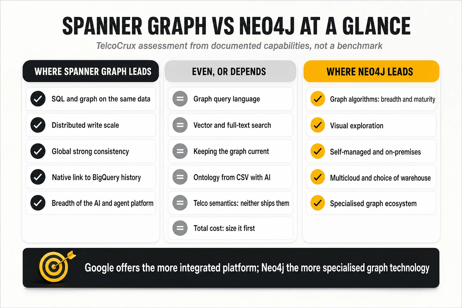
Spanner Graph versus Neo4j, dimension by dimension. Assessments are TelcoCrux views from documented capabilities as of October 2026, not benchmark results.

At a glance: Google offers the more integrated platform; Neo4j the more specialised graph technology. A summary of the matrix above.

Time to the first use case: a packaged path versus a toolkit

The matrix compares capabilities; it does not show how much work separates the operator from its first useful result. On that question the two offers differ more than on any technical dimension.

Google sells a path, not only a database. Its Autonomous Network Operations framework is specific to telecom: a reference design, a progression from model to shadow to twin, worked examples built on network data, notebooks for loading and querying, an ontology assistant, the history, graph learning and agent layers already wired to each other, and a team and partners that have run pilots with operators. An operator can go from a folder of exports to a working demonstration of root cause and impact on its own data in weeks, with the supplier alongside. That accompaniment is a real advantage when the organisation’s first question is “show me it works here”.

Neo4j sells the strongest graph toolkit, and the path to the use case is more the operator’s to build. For the questions that are purely about the graph — dependencies, impact, paths, single points of failure, visual exploration — reaching a result is just as fast, and in structural analytics faster, because the algorithms are ready and mature. What is not packaged in the same way is everything around the graph: the warehouse, the streaming pipelines, the predictive models and the orchestration of agents are chosen and integrated by the operator or a systems integrator. Neo4j’s offer is cross-industry rather than a telco-specific operations framework; its telecom expertise comes through references and partners such as the integrators behind the BT and Sopra Steria solutions, not through a packaged autonomous network kit.

Question	Google Cloud	Neo4j
Telco-specific framework	Yes: Autonomous Network Operations	No: cross-industry platform with telecom references
What comes pre-connected	Graph, history, graph learning, agents, ontology assistant	Graph, graph analytics, GraphRAG and agent tooling
What the operator or integrator assembles	Feeds from its own systems; the ontology review	Feeds; plus warehouse, pipelines, predictive models and agent orchestration
Fastest to demonstrate	End-to-end root cause, impact and agents on Google Cloud	Dependencies, impact and structural vulnerabilities
Main risk of the easy path	Adopting the whole stack because the first result was convenient	Underestimating the integration needed beyond the graph

Time to the first use case. A TelcoCrux assessment of what each offer brings ready-made, and what the operator still has to build.

Two cautions keep this honest. A demonstration prepared by a supplier on its own environment is not the operator’s network; the fair test is to give both suppliers, or their integrators, the same exports and the same twenty questions and compare what comes back, in the same number of weeks. And ease at the start is not the same as the right platform for ten years: the convenience of a packaged path should be weighed against concentration in one supplier, and the freedom of a toolkit against the engineering it requires.

What changed in 2026

A year earlier, this comparison would have been more lopsided in both directions. Four releases moved it.

Spanner Graph algorithms (preview, June 2026) gave Google managed centrality, clustering, similarity and path algorithms on independent compute. That removed the strongest argument that Spanner had no graph analytics; Neo4j still has the longer track record and broader catalogue.
Graph types in Neo4j (GA, June 2026) brought enforceable structure to a schema-flexible engine, answering the governance objection that large operators raised against it.
Infinigraph (December 2025) gave Neo4j property sharding for very large graphs, narrowing — not closing — the distributed scale gap, with licensing and deployment caveats.
Aura Agent (GA, February 2026) and the official MCP server gave Neo4j its own path to graph-grounded agents, while Google’s agent platform remains broader for full autonomous operations.

Six NOC decisions, six verdicts

Abstract matrices help less than concrete decisions. The six below are the ones that most often justify a twin in a network operations or security operations centre.

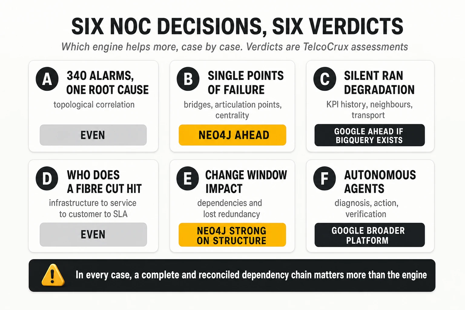
Six NOC decisions and the engine that helps more in each. In every case, a complete and reconciled dependency chain matters more than the engine.

A. Correlating 340 alarms and locating the root cause

Both engines can traverse the topology and find that apparently independent alarms share a router, an optical link or a network function. Verdict: a functional tie, subject to latency and model quality. A graph reveals dependencies and supports hypotheses about root cause; it does not prove causality by itself. That needs time sequences, states, rules and operational evidence.

B. Finding single points of failure before an incident

This is an algorithmic problem: bridges, articulation points, centrality and loss of redundancy. Verdict: Neo4j ahead, through the maturity and breadth of Graph Data Science, where these algorithms are production-grade. Spanner can address part of the problem with its current algorithms; check which functions exist and their availability stage.

C. Anticipating silent degradation in the RAN

It requires combining KPI history, cell states, neighbour relations, congestion and transport relationships. Verdict: a potential advantage for Google’s integration where BigQuery and its ML platform already hold the history. Neo4j is viable too, with GDS embeddings, external GNNs and a warehouse. The result will depend more on the predictive model and the training data than on the database.

D. Identifying the services and customers hit by a fibre cut

It needs a traversal from physical infrastructure through logical transport to services, customers and service-level commitments. Verdict: a functional tie. What decides the outcome is having a complete, reconciled dependency chain, not the engine.

E. Simulating the impact of a change window

Both can identify dependencies, alternatives and resources that would lose redundancy. Verdict: Neo4j is very attractive for the structural analysis, but both need a model of network behaviour. Computing paths on a graph is not the same as verifying real forwarding, convergence, post-change utilisation or routing policy; controllers and model-based verification tools (family 4 in section 5) have to contribute there.

F. Autonomous diagnosis and resolution agents

Google brings an integrated ecosystem of models, agent runtime, connectors and data tools; Neo4j brings specialised, structured access to network knowledge through MCP and GraphRAG. Verdict: Google has the broader platform, and Neo4j can be part of it. Action control, policies, checks and the approval loop must be built in both cases.

What the public evidence actually shows

The public references are relevant and not directly comparable.

Neo4j: BT Group’s wholesale inventory twin publishes operational metrics (60% fewer human decision points, 50% less capacity-planning time); Comcast has described a nationwide network twin in production without comparable figures.
Google: a 2026 proof of concept with MasOrange and NetAI shows a Spanner Graph twin with billions of dependencies and a GNN for root cause, demonstrating architecture and scale within the communicated scope, without production results.

None of this allows a winner to be declared on performance, cost or root cause precision for a specific national network. A production deployment described at a conference and a proof of concept answer different questions, and vendor customer stories are not independent audits.

Cost, operations and supplier dependence

The database is often a small part of the cost of a network twin. Initial integration, inventory reconciliation, maintaining the feeds and operating the model typically cost much more. Licences and infrastructure still matter, and they are priced on different bases.

Neo4j AuraDB is priced per GB of provisioned memory per hour: $0.09 for Professional and $0.20 for Business Critical, with a 2 GB minimum and a 99.95% SLA on Business Critical; dedicated and self-managed options are priced commercially; Aura Graph Analytics sessions cost $0.40 per GB per hour.
Spanner requires sizing the Enterprise or Enterprise Plus edition, processing units, storage, Data Boost compute for algorithms, BigQuery and any other services used; Enterprise Plus multi-region configurations offer an SLA of up to 99.999%.

Those SLAs are not equivalent unless the contracted architectures are. A fair comparison needs a three-year total cost of ownership under the same volume, availability, regions, performance and workload. And sovereignty is a strategic difference, not a line item: Neo4j can run in the operator’s own data centres, while Spanner Graph is tied to Google Cloud. Where policy requires critical topology data to stay on premises, that can decide the matter before any benchmark is run.

Three architectures worth evaluating

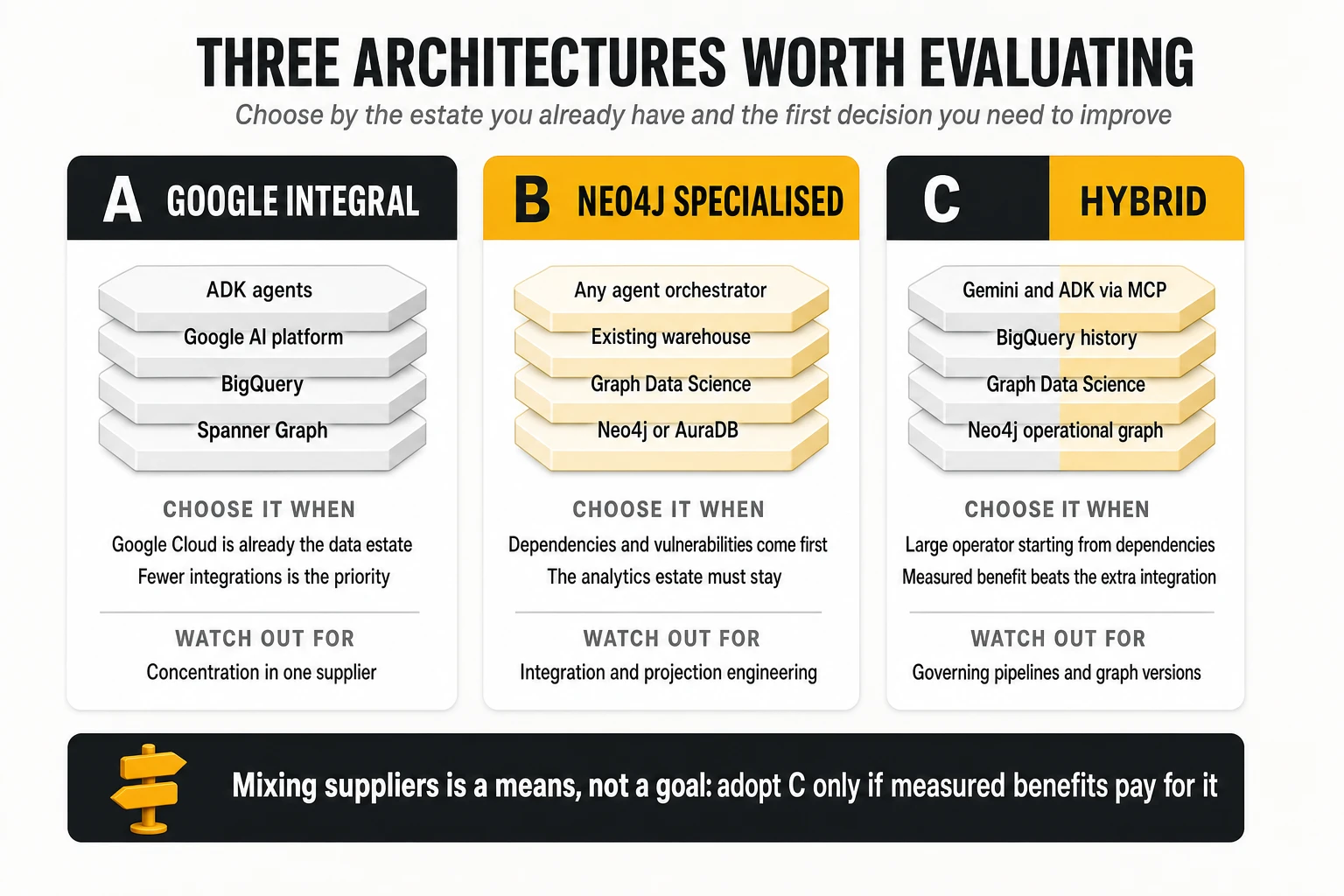
Architecture A: Google integral

Spanner Graph, BigQuery, Google’s AI platform and ADK agents. Choose it when the operator already uses Google Cloud intensively, manages large relational datasets and values fewer integrations between components. Watch for concentration in one supplier, and verify the cost and the maturity of the graph engine on the most demanding query patterns.

Architecture B: Neo4j specialised

Neo4j or AuraDB, Graph Data Science, the existing warehouse and an agent orchestrator of choice. Choose it when the priority is a connected inventory, dependencies, topological correlation, vulnerabilities and graph algorithms — especially if a corporate analytics estate exists that should not be replaced. Watch for the engineering needed to integrate the components and operate the analytics projections.

Architecture C: hybrid

A Neo4j operational graph with GDS, BigQuery for history and Gemini with ADK agents reaching the graph through MCP. This is the architecture TelcoCrux would most like to see evaluated in a large operator that starts from network dependencies: it uses Neo4j’s graph specialisation, Google’s analytics and ML services, and keeps the agent layer independent of the data engine. Its risk is governance of the pipelines, the graph versions and the coherence between systems. Adopt it only if Neo4j’s measured benefits exceed the cost of the extra integration — never as an aesthetic preference for mixing suppliers. A fully self-managed Neo4j variant with an existing analytics platform is a fourth option where data residency justifies it.

How to decide

If the main goal is an operational graph to improve correlation, impact assessment and vulnerability analysis, start by evaluating Neo4j: its ecosystem is built for complex relationships, its algorithm library is mature and it has relevant telecom references.
If the goal is a distributed operational data and AI platform of corporate scope, especially on Google Cloud, Spanner Graph deserves the first evaluation: its advantage is combining the graph with relational capabilities and deep integration with history, ML and agents.
If the operator already runs topological correlators and graph databases, replace nothing until it is shown what new capability the alternative brings. The value is more likely to lie in extending the model across domains, linking services and customers, adding history and improving decisions — whichever engine is chosen.

Before asking whether Spanner is better than Neo4j, an operator should ask which information and which decisions it cannot connect today. That answer should determine the pilot, the test queries and, finally, the technology. An incomplete topology in the best database in the world will still produce incomplete diagnoses: dependency coverage, key quality, continuous updating and the resource-service-customer chain are the real conditions of success.

10. What the twin can answer once it is loaded

Once loaded, a graph-based twin answers questions at six levels of difficulty. The first four are deterministic graph queries. The fifth adds search over text and meaning — keyword and vector search combined with the graph — which needs indexes and embeddings but no model trained on the operator’s incidents. Only the sixth is learned inference, the GNN layer of section 2. Most of the operational value sits in levels two to four, which is also where existing tools are weakest.

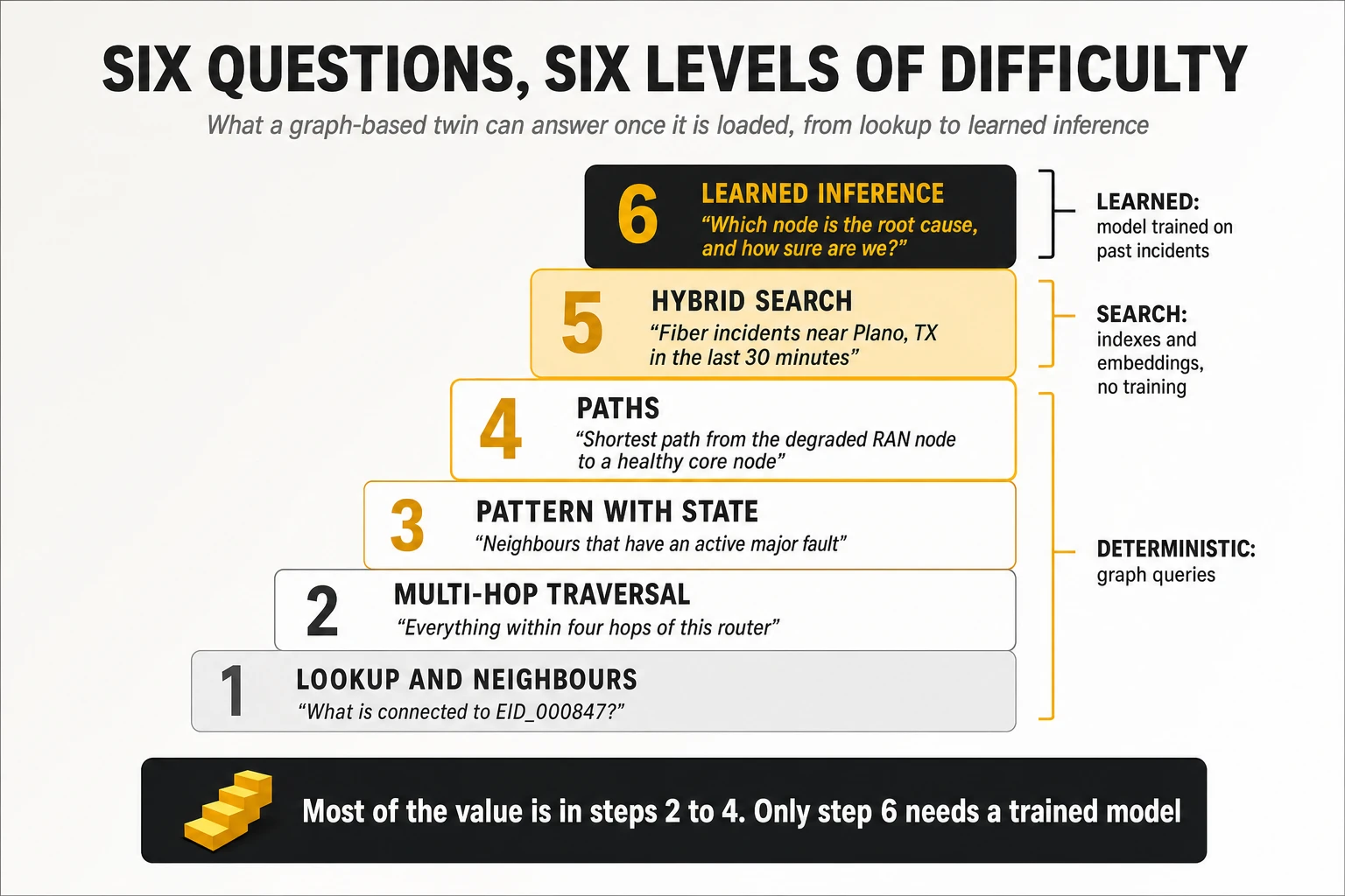
Six levels of questions. Levels 1 to 4 are deterministic graph queries; level 5 adds text and semantic search without any training on the operator’s data; level 6 is learned inference, which earns its cost only where the others run out.

Level	Example question	How the twin answers	Typical consumer
1. Lookup and neighbours	What is EID_000847 connected to?	One-hop pattern match	NOC engineer, field technician
2. Multi-hop traversal	Everything within four hops of this aggregation router	Variable-length path, 1 to 4 hops	Impact assessment, change planning
3. Pattern with state	Which neighbours have an active major fault?	Graph pattern plus filters on fault properties	Incident triage and correlation
4. Paths	Shortest path from the degraded radio node to a healthy core node; all paths between two faulty nodes	Path search with constraints	Root cause, rerouting, redundancy checks
5. Hybrid search	Fibre-related incidents near Plano, TX in the last 30 minutes, on elements serving this enterprise	Full-text or vector search combined with graph and time filters; no trained model	Agents, NOC chat, service desk
6. Learned inference	Which node is the probable root cause, with what confidence, and what is the business impact?	Graph neural network trained on past incidents, applied to the current subgraph	Automated triage, closed-loop assurance

The ladder of questions. Each level reuses the twin built for the previous one; nothing new has to be loaded to move from level 1 to level 4.

Agents change who can ask, not what can be answered. A conversational agent translates “what is this switch connected to, expand two hops, show the shortest path between the two faulty ones” into level 1, 2 and 4 queries. That democratises the twin for operations and field staff who do not write graph queries, and it makes every answer traceable to a query that can be inspected.

11. Seven practical cases on illustrative US data

The cases below show the twin at work on problems operators actually have. Locations are real US places; identifiers, topologies and figures are fictional and illustrative unless a source is given. Each case states what is deterministic and what, if anything, requires a learned model. All seven can be built on either Spanner Graph or Neo4j; where one engine has a clear advantage, section 9 says so.

Case 1. A chronic radio degradation and its reach into the core (Dallas – Fort Worth)

Situation. Several cells around Plano, Texas, have shown chronic performance degradation for weeks without a hard alarm severe enough to trigger a ticket. Separately, two core nodes in Dallas carry active faults. Nobody has asked whether they are related, because they sit in different teams’ consoles.

How the twin answers. Three queries, all deterministic.

Find the radio nodes with the oldest active degradation (the ranking query in section 6): the oldest, EID_000063, has been degraded since late May.
Walk one to four hops upward from that node and return core nodes with active faults: two core nodes in Dallas appear on the paths, through two aggregation nodes.
Return the shortest path from the degraded radio node to a healthy core node: a three-hop path to a core node in Houston exists, which tells the planner a reroute is possible.

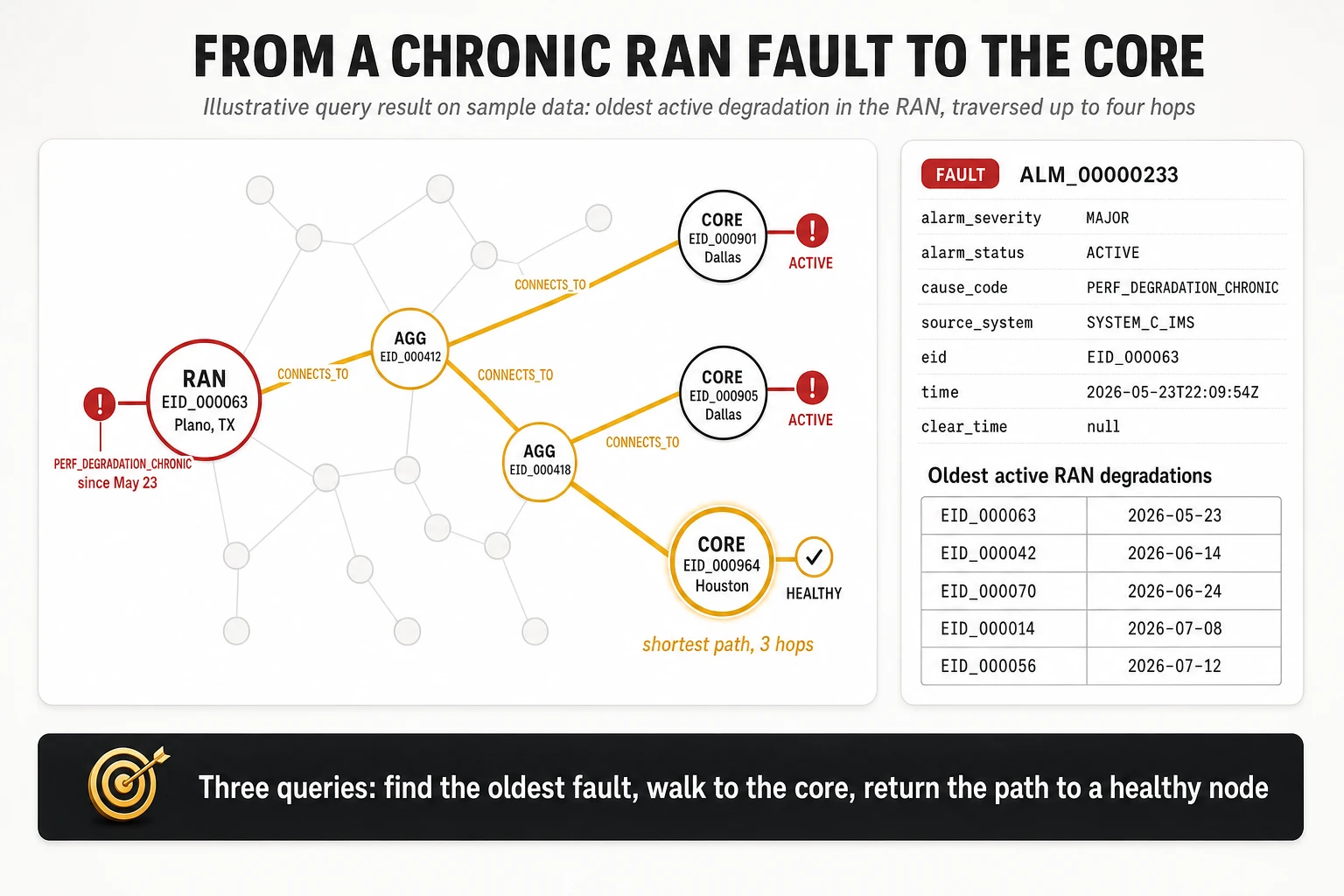
From a chronic radio fault to the core. Three queries — find the oldest fault, walk to the core, return the path to a healthy node — turn two unrelated console entries into one hypothesis. Illustrative data.

What it changes. Two queues become one investigation with a shared hypothesis and a candidate mitigation. The twin does not prove causation; it shows that the elements are connected and both degraded, which is the question no single console could answer.

Case 2. A new element appears, and the graph sees it immediately

Situation. A field team commissions a new aggregation switch next to EID_000847, and the inventory system records it, together with an alarm raised during commissioning.

How the twin answers. The inventory feed inserts a row into the entity table, a row into the entity-to-entity table and a row into the faults table, in one transaction. The next neighbourhood query around EID_000847 returns four neighbours instead of three, one of them with a fault edge. No rebuild, no re-indexing job.

What it changes. This is the concrete meaning of “real-time topology”: the graph is exactly as current as the sources that write to it. It also exposes the dependency honestly — if the inventory is updated a week late, the twin is a week late.

Case 3. A backhaul fibre cut in North New Jersey, ranked by business impact

Situation. In an illustrative scenario, a backhaul fibre is cut in a revenue-dense area of North New Jersey. Alarms arrive from radio sites, transport and aggregation. The operator has a business intent registered through a TM Forum TMF921 intent interface: assure mobile broadband customer experience in these zones, decomposed into service expectations for throughput, latency, availability and quality of experience.

How the twin answers. The failure is written to the graph; a reflex agent detects the breach of the intent; a GNN trained on the twin’s history ranks probable origins. The ranking combines model confidence with business weight — cell profile, revenue density and time of day — rather than counting alarms. The sequence then hands over to diagnosis, execution of a backhaul reroute through the controller, and a reflection agent that verifies the intent’s expectations are met again before closing the loop.

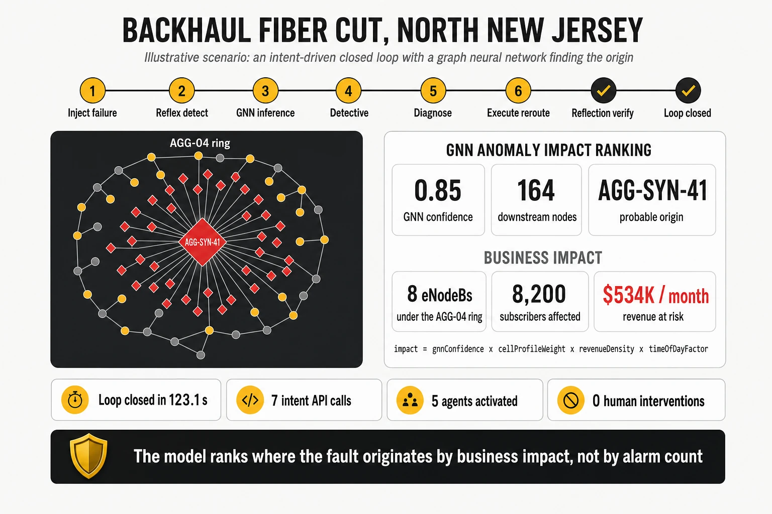
A closed loop in an illustrative scenario: the GNN names the probable origin and ranks it by business impact, and agents reroute and verify. Every figure is illustrative, not an operator measurement.

Indicator (illustrative data)	Value
GNN confidence in the probable origin (AGG-SYN-41)	0.85
Downstream nodes in the blast radius	164
4G base stations (eNodeBs) under the affected aggregation ring	8
Subscribers affected	8,200
Revenue at risk	USD 534,000 per month
Time to close the loop	123.1 seconds
Intent API calls / agents activated / human interventions	7 / 5 / 0

The scenario’s outputs. They illustrate the shape of the result — origin, impact in business terms, verified closure — and should not be read as performance benchmarks.

What is deterministic and what is not. For a clean fibre cut on a known ring, a topology rule would also find the span; this case is honest only if the value claimed is the ranking by business impact and the automated, verified closure, not the localisation itself.

Case 4. Attach failures on game night (Arlington, Texas)

Situation. During a championship game at a 70,000-seat stadium, smartphones near the venue fail to attach to the network. Two hypotheses compete: the stadium cells are congested because two of the three sectors on the main site have failed, or the subscriber database behind the mobility management function is unreachable.

How the twin answers. The control and user plane are already a graph: device, radio node, mobility management (MME in 4G, AMF in 5G), subscriber database (HSS or UDM), serving and packet gateways. The shape of the failures on that graph separates the hypotheses. If attach failures are confined to cells sharing the stadium site while neighbouring cells on the same MME are normal, the problem is radio and capacity. If failures spread across every cell served by that MME and the S6a interface shows timeouts, the problem is the database.

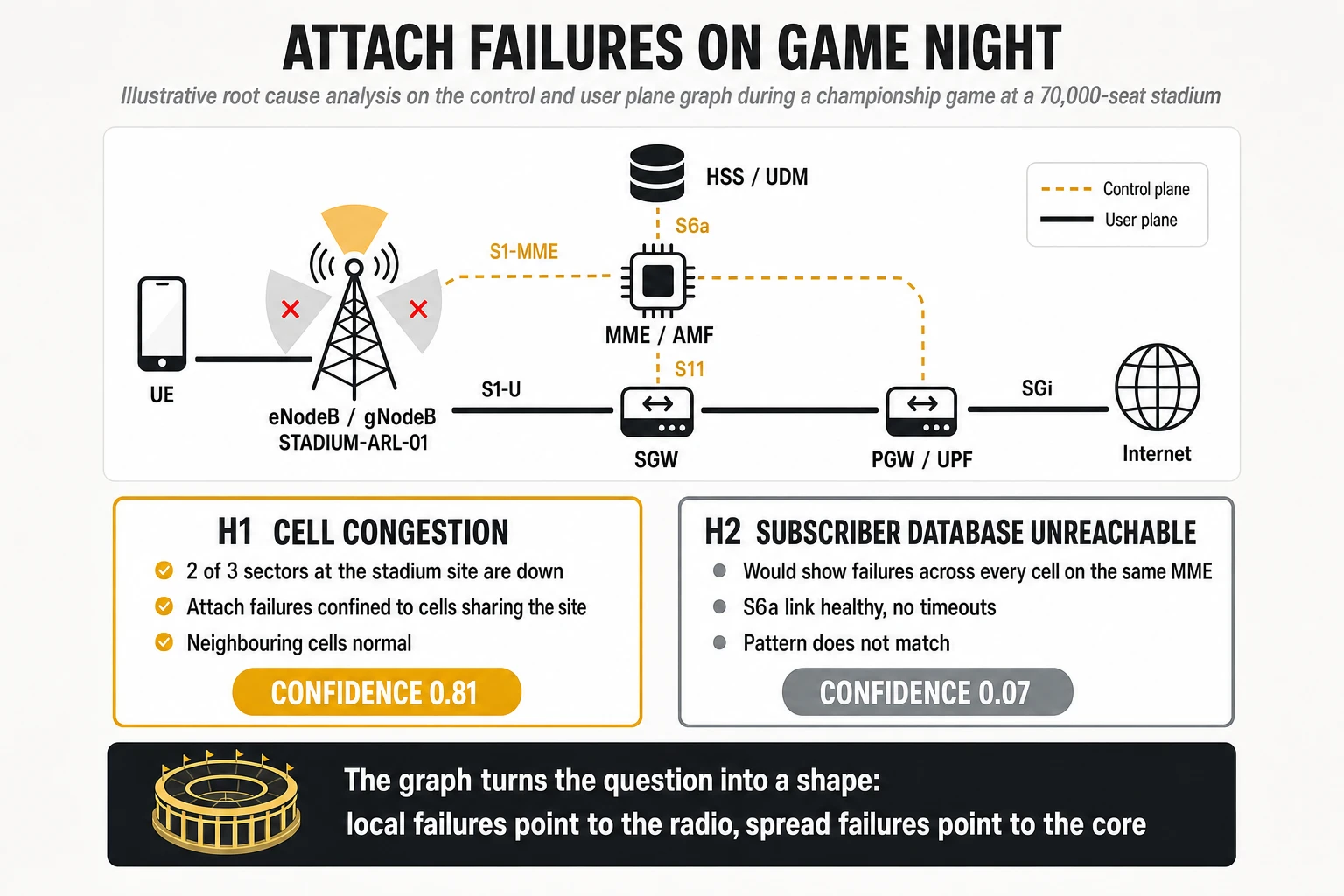
Game night: the graph turns the question into a shape. Local failures point to the radio; failures spread across the MME’s footprint point to the core. Illustrative data and confidence values.

What it changes. The right team is paged in the first minutes rather than after a war room has formed. A learned model adds value before the event rather than during it: trained on previous large events, it can predict which cells and which backhaul links will saturate, and which cells some distance from the stadium will degrade through shared transport — the kind of cascade that is obvious in hindsight and invisible in advance.

Case 5. Mobility on the I-95 corridor

Situation. Customers complain of dropped calls and stalled sessions on the stretch of I-95 between New York and Boston. Drive tests are expensive and quickly out of date.

How the twin answers. Daily handover counts between every pair of neighbouring cells are loaded as weighted edges; cells are linked to the corridor they cover. A query along the corridor returns the sequence of handovers a car at highway speed actually traverses, with success rates per edge. One weak edge near New Haven stands out at 91% while its neighbours sit around 98-99%. Historical alarms and configuration changes on the cells at either end are one hop away.

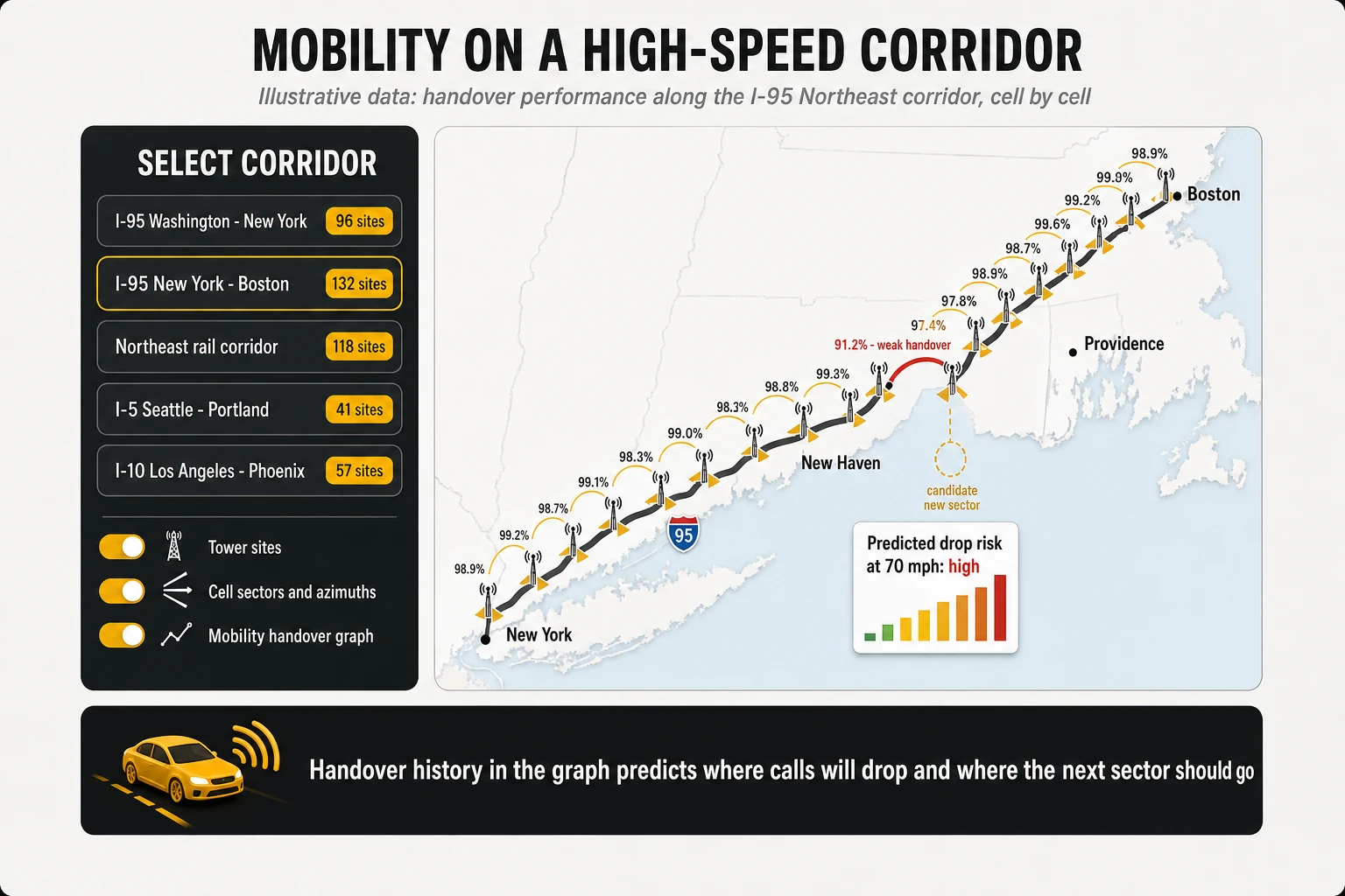
Mobility as a graph: handover history along I-95 shows where sessions drop and where a new sector would help. Site counts, percentages and predictions are illustrative.

What learning adds. With months of handover and KPI history, a model can predict which corridor segments will degrade under holiday traffic and rank candidate locations for a new sector by the handover edges it would repair. This is a planning use case, and it is where a twin starts to pay for capacity investment rather than only for operations.

Case 6. Before the change window: what depends on this router?

Situation. A software upgrade is planned on an aggregation router in the Chicago metro area. The change request lists the router; it does not list what depends on it.

How the twin answers. A traversal from the router collects the cells it backhauls, the enterprise services whose paths cross it, and the elements whose only redundant path runs through it. Two checks follow: is any of the redundant paths already in a maintenance window or carrying an active fault, and which enterprise customers with service commitments would lose redundancy during the upgrade?

What it changes. The blast radius is computed before the window opens rather than discovered during it. Run continuously rather than per change, the same question becomes the structural analysis of section 7: articulation points and bridges computed over the whole topology flag in advance which routers should never be upgraded without first adding a diverse path. Combined with change records stored in the twin, this is also how an operator learns that a recurring class of incidents follows a recurring class of change.

Case 7. Switching cells off without losing coverage

Situation. At night, traffic in suburban areas falls far below capacity, and capacity layers could be put to sleep to save energy — if doing so does not leave anyone without coverage or overload the remaining cells.

How the twin answers. Cells that overlap in coverage are linked by edges carrying measured overlap and handover volume; energy and traffic counters are properties. A query returns, per area, the capacity cells whose traffic can be absorbed by neighbours that remain awake, and excludes cells serving commitments such as emergency services or enterprise sites. A forecast of demand — including known events — decides when to wake them.

What it changes. Energy saving becomes a decision constrained by the network’s structure and by commitments, rather than a static schedule. It is also a case where the twin’s return path — the controller actually switching cells — is low risk and easy to verify, which makes it a good first candidate for closed-loop automation.

The seven cases at a glance

Case	Question	Deterministic part	What a model adds	Value
1. Chronic RAN to core	Are these faults related?	Traversal and paths	Not required	Two queues become one investigation
2. New element	Is the topology current?	Transactional update	Not required	Real-time context, as current as the feeds
3. Fibre cut, New Jersey	Where did it start, and what does it cost?	Localisation on a known ring	Ranking by business impact; automated closure	Prioritisation by revenue and customers
4. Game night	Radio or core?	Failure shape on the graph	Prediction of saturation and cascades before the event	Right team in minutes; preventive action
5. I-95 corridor	Where do sessions drop, and where to build?	Handover edges along the route	Prediction of degradation; ranking of new sectors	Better capacity investment
6. Before a change	What depends on this router?	Blast radius and redundancy	Learning which changes cause incidents	Fewer change-induced outages
7. Cell sleep	Which cells can sleep safely?	Coverage overlap and commitments	Demand forecast	Energy savings without coverage loss

Most of the value in the seven cases comes from deterministic graph queries. Learned models add value in five of them, and in each for a specific reason: ranking by impact, prediction, planning or learning from history.

12. Limits, risks and where the hype is

A network twin is a sound idea that is easy to oversell. The risks below are ordered by how often they decide the outcome of a programme, not by how often they appear in vendor slides.

1. The model is the product, and it belongs to the operator

The single largest risk is treating the ontology as a deliverable of the supplier. No vendor arrives with a telco model that fits; the operator’s engineers have to own the definitions of entities, keys and relationships, and keep owning them as the network changes. Programmes that outsource the model end up with a twin nobody inside trusts.

2. Freshness depends on feeds nobody budgeted

The graph is as current as the last row written. The CSV route produces a convincing demonstration in weeks; the integrations that keep it current — inventory events, controller APIs, fault streams — are the slow, unglamorous part. A twin that drifts from the network is worse than no twin, because it is believed.

3. Deterministic tools already solve the easy cases

A fibre cut on a known ring, a power failure at a site, a card failure with clear alarms: topology-aware rules already handle these. A programme justified by such cases will be correctly challenged on cost. The business case must rest on what determinism cannot do — silent degradations, cascades, ranking by impact, prediction and planning — and must be measured against the operator’s current results, not against a manual baseline.

4. Learned models need history, labels and humility

A graph neural network trained on three months of poorly labelled incidents will produce confident, unreliable rankings. Models need months of history, consistent incident labels, and evaluation on held-out incidents before they influence a decision. Confidence values must be shown to engineers, and the model’s precision tracked per incident class.

5. The engine debate is real but secondary

Operators with existing graph databases in production will ask whether a new engine is needed, and vendors will ask them to choose between Spanner Graph and Neo4j. The functional vision — dependencies plus live state plus traversal — is the same across engines; section 9 shows that the differences are real but sit in operational characteristics: consistency, scale, graph analytics, multi-model support, integration with history and machine learning, deployment model, cost and lock-in. That is a technical evaluation to run on the operator’s heaviest queries, not a reason to delay the functional work. The engine choice should not absorb the attention that the dependency chain deserves.

6. Cost, sovereignty and lock-in

Higher database editions, analytical reservations, model training and agent usage add up. Topology and customer mappings are sensitive data with residency implications. Standard query languages (GQL, SQL/PGQ), the operator’s ownership of the model, and exportable tables mitigate lock-in; they do not remove it.

7. Agents multiply the value and the risk

An agent with access to the twin answers better; an agent with access to the controllers can also do damage. Read-only first, typed tools with explicit permissions, actions classified by risk and an audit trail of every query and action are prerequisites, not refinements.

13. A pilot that proves or kills the idea, and a fair benchmark

The right first step is a bounded pilot with success and kill criteria written before the first file is loaded. Ten weeks is enough to know whether the twin answers questions the operations centre cannot answer today.

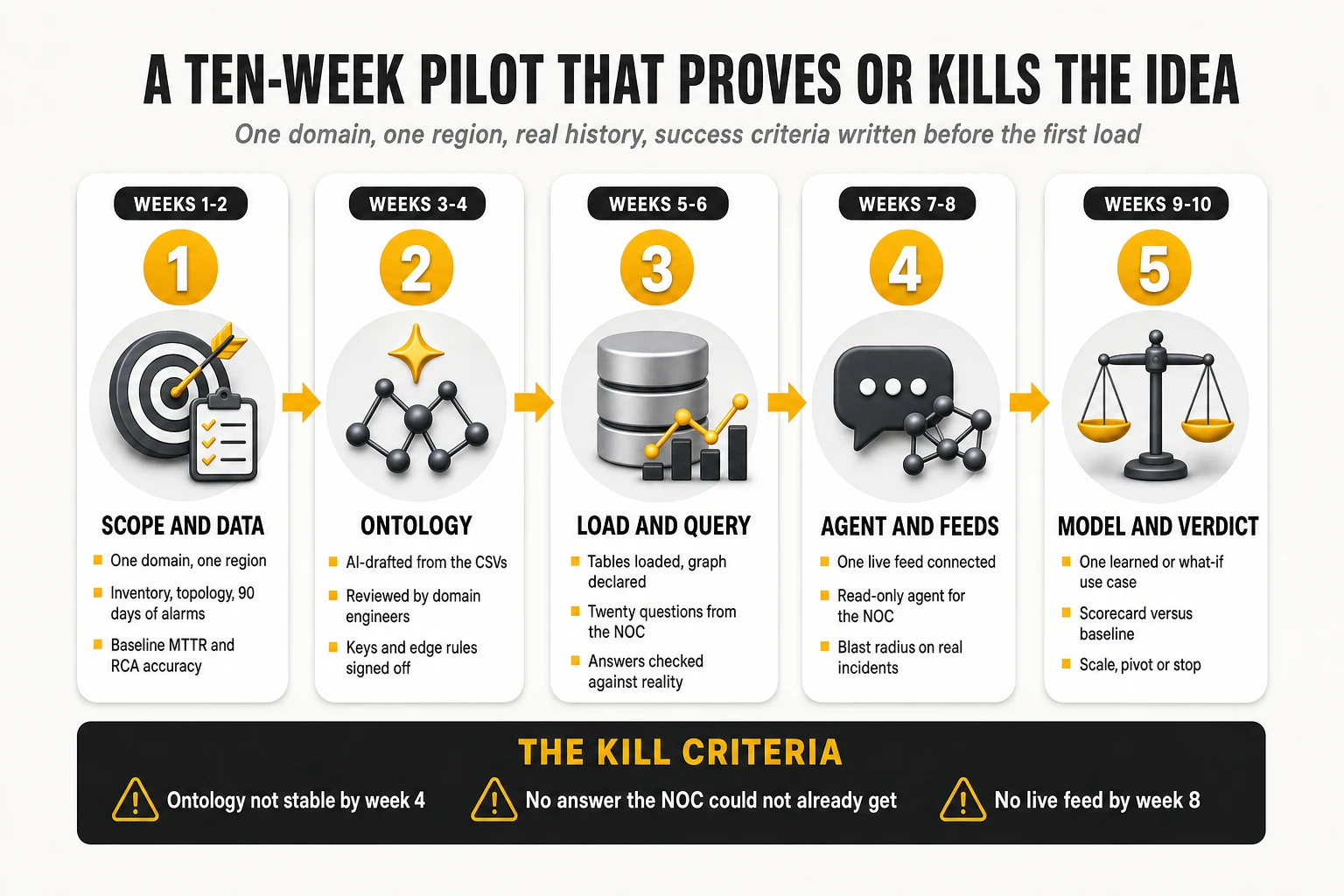
A ten-week pilot with explicit kill criteria: an unstable ontology by week 4, no answer the operations centre could not already get, or no live feed by week 8.

Weeks	Phase	Deliverable	Gate
1-2	Scope and data	One domain and one region chosen by data availability; inventory, topology, 90 days or more of alarms, KPIs, tickets and changes exported; current mean time to repair (MTTR) and root cause accuracy measured	Data delivered and baseline recorded
3-4	Ontology	AI-drafted model from the CSV files; review sessions with domain engineers; keys and edge rules signed off	Model stable; validation facts agreed
5-6	Load and query	Data loaded and graph built; twenty questions supplied by the operations centre answered and checked against reality	At least half the questions answered better or faster than today
7-8	Agent and feeds	One live feed (fault or inventory events) connected; read-only conversational agent for the operations centre; blast radius computed on real incidents	Live updates visible; engineers using the agent unprompted
9-10	Model and verdict	One learned or what-if use case (impact ranking, prediction or pre-change analysis) evaluated on held-out incidents; scorecard against baseline	Decision: scale, pivot or stop

The pilot plan. Choosing the domain by data availability matters more than choosing it by ambition: some operators start with fixed networks, others with radio, depending on where history and inventory are cleanest.

Measure outcomes, not activity. The scorecard should report time to identify the probable origin, share of incidents where the twin’s top hypothesis was correct, time to establish affected services and customers, number of questions answered that could not be answered before, model freshness after changes, and the engineering effort spent per new data source. Loaded tables, nodes counted and agents deployed are inputs.

A fair head-to-head benchmark

When the shortlist has two engines, the pilot should run them side by side on exactly the same data and the same questions. A test on ten thousand synthetic routers is useful to learn a query language and useless for choosing the architecture of a national network: the load must look like production, with highly connected nodes, cross-domain relationships and concurrent events.

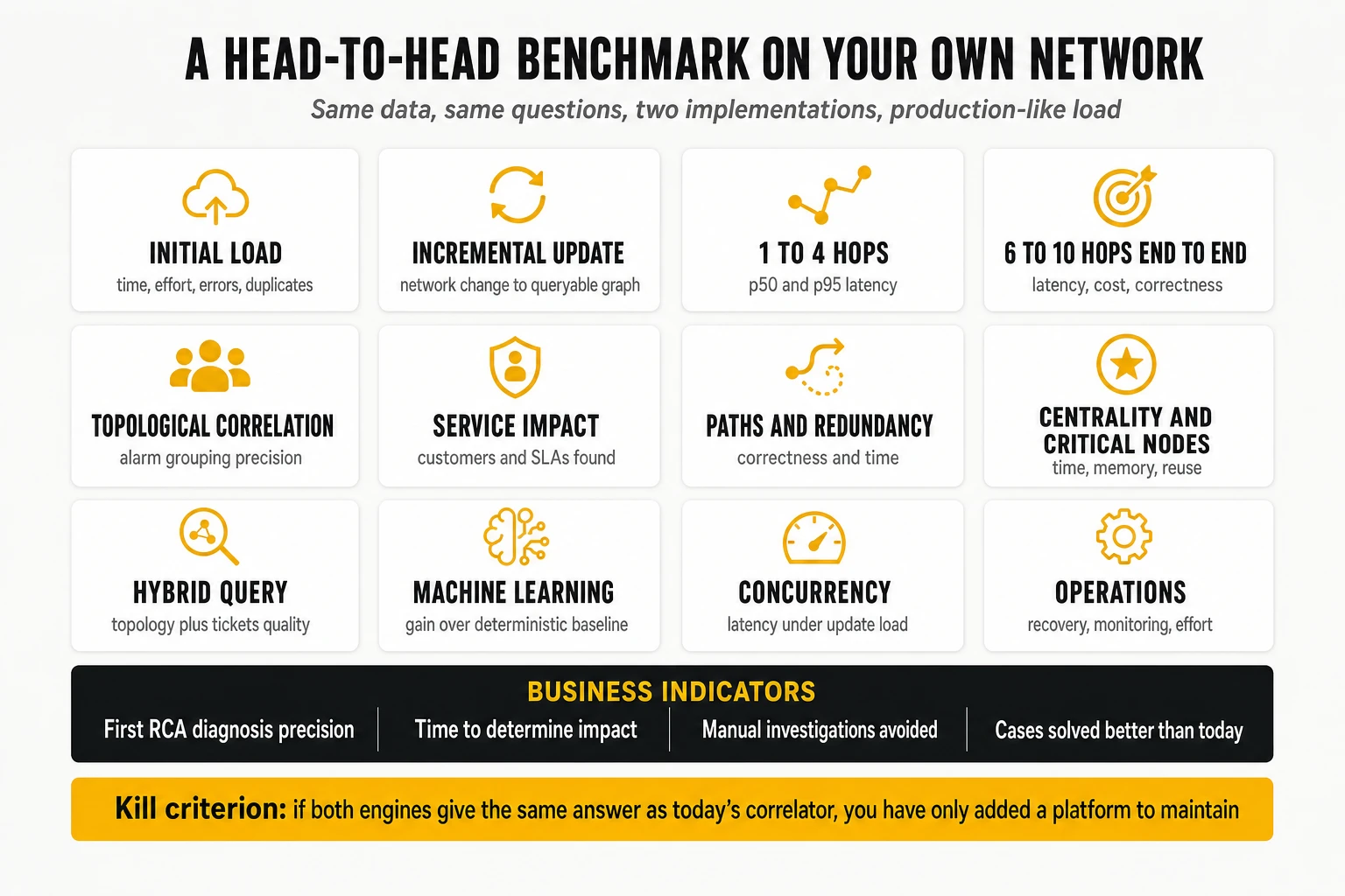
A head-to-head benchmark on the operator’s own network: same data, same questions, two implementations, production-like load, and a kill criterion.

Test	What to measure
Initial inventory load	Time, effort, errors and duplicates
Incremental update	Real latency from a network change to a queryable graph
Neighbourhood of 1 to 4 hops	p50 and p95 query latency
End-to-end dependencies of 6 to 10 hops	Latency, resource consumption, correct results
Topological correlation	Precision of alarm grouping
Service impact	Customers and SLAs correctly identified
Paths and redundancy	Correctness and computation time
Centrality and critical points	Time, memory, reuse of results
Hybrid query	Quality of answers combining topology and tickets
Machine learning	Improvement over the deterministic baseline
Concurrent queries	Latency under a load of updates
Operations	Recovery, monitoring and maintenance effort

A head-to-head benchmark matrix. Each test runs on both implementations, on the same data and topology, under production-like concurrency.

Measure the path as well as the engine. Give both suppliers, or their integrators, the same exports, the same twenty questions and the same number of weeks, and record how much of the result came packaged and how much the operator’s team had to build. That separates the convenience of a supplier-led demonstration from the effort of running the twin in production.

Four business indicators decide the verdict: precision of the first root cause diagnosis, time to determine impact, reduction in manual investigations, and the share of cases the graph resolves better than the engines already in place. One discard condition is essential: if both engines give the same answer as the current correlator and add a platform to maintain, the project has not proved its value. The benefits must show up in end-to-end coverage, inventory quality, commercial impact, handling of uncertainty, prediction or preventive decisions.

What each type of operator should do

Large operators with existing graph tools: do not replace what works. Run the pilot on a domain the current graphs do not cover, or on a use case they cannot serve — structural vulnerability analysis, impact ranking, prediction, hybrid search — and evaluate engines on that use case, with the head-to-head benchmark above.
Operators with sovereignty constraints on topology data: the deployment model narrows the field before any benchmark. A self-managed graph platform on premises, with cloud services used only for non-sensitive analytics, may be the only compliant design.
Mid-sized operators without a consolidated inventory: the CSV route doubles as an inventory consolidation exercise. Use it to build the first connected inventory for one domain, and decide afterwards whether the twin becomes the system of record for parts of the estate.
Operators with a cloud data platform already in place: the twin is an extension of the existing estate. Start where history already lives, add the operational graph and the native integrations, and keep the agent layer read-only until the twin has earned trust.

14. Conclusions

First, a network digital twin for operations is a graph of the network joined to its live state and its history. It is not a 3D model or a simulator in the first instance. Its job is to supply context — the dependency chain, the affected services, the memory of changes and incidents — that monitoring and observability tools collect evidence for but cannot provide.

Second, the shadow is the level that matters. A static model is an inventory with a better query language; a full twin with trusted simulation and a closed loop is years away for most domains. A shadow kept current by real feeds is where root cause analysis, impact assessment and grounded agents become possible.

Third, the economics changed at the modelling step. AI-assisted ontology from flat exports collapses the time to a first useful model from quarters to weeks. It does not remove the review, the feeds or the ownership of the model, and anyone presenting it as plug-and-play is selling the demonstration rather than the programme.

Fourth, the two leading approaches solve the same problem from opposite ends. Google declares the graph over relational tables in a strongly consistent, distributed, multi-model database and connects it natively to BigQuery for history, to graph neural network tooling for learning and to a broad agent platform. Neo4j stores the network as a native graph and surrounds it with the most mature graph analytics library in the comparison, graph-grounded generative AI, agent tooling through MCP, and the freedom to run on any cloud or on premises with any warehouse. Google offers the more integrated platform and a packaged, telco-specific path to the first use cases; Neo4j offers the more specialised graph technology, with a path that the operator or its integrator builds. Neither ships telco semantics, neither discovers the network, and neither has published the kind of independent before-and-after evidence that would settle the choice in general.

Fifth, the choice should follow the operator’s situation, not the vendors’ slides. Start with Neo4j when the first goal is dependencies, correlation, impact and structural vulnerabilities, or when topology must stay on premises; start with Spanner Graph when the goal is a corporate operational data and AI platform on Google Cloud, or when the fastest supplier-led path to a first end-to-end use case matters most; consider the hybrid only if measured benefits pay for the extra integration; and decide with a head-to-head benchmark on the operator’s own data.

Sixth, most of the value is deterministic, and learning must be justified where determinism ends. Traversals, paths and patterns with state deliver the bulk of the benefit, and graph algorithms add structural intelligence — single points of failure, critical links, clusters — without any learned model. Learned models earn their cost in ranking by business impact, prediction and planning, and only after they have been measured on the operator’s own incidents.

A twin earns its place when it answers a question the operations centre could not answer the day before. Build it on one domain, from the data that already exists, with the operator’s engineers owning the model; measure it against the tools already in place; and extend it only as far as the evidence supports.

At TelcoCrux, we help operators decide whether a network digital twin answers questions their current tools cannot, and on which platform: which domain to start with, which data to export, how to compare Spanner Graph, Neo4j or a hybrid on the operator’s own queries, how to design a pilot and a head-to-head benchmark with honest kill criteria, and where graph algorithms or learned models are worth their cost. If you are evaluating a graph-based twin for assurance or autonomous operations and want an independent read before committing, let’s talk.