AI Is Making Physical Network Infrastructure Scarce Again

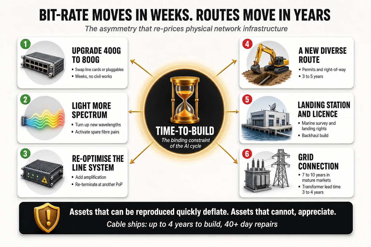
Upgrading a live 400G wavelength to 800G is an engineering exercise measured in weeks: new line cards or coherent pluggables at each end, a maintenance window, a re-optimised optical line system. Building a new, physically diverse route between those same two points — permits, right-of-way negotiations, civil works, a cable landing station, a grid connection — is measured in years. The gap between the timeline of the electronics and the timeline of the trench is the most important number in AI infrastructure today, and it appears on no transceiver datasheet.

The prevailing narrative compresses four distinct phenomena into a single sentence: “AI needs a lot of fibre.” AI training traffic, general cloud traffic, optical transmission economics and infrastructure ownership are four separate curves with different drivers, different geographies and different time constants. Treating them as one produces the two failure modes visible across the industry right now — capacity plans that over-provision the wrong segment, and investment cases that price kilometres of glass instead of pricing scarce routes.

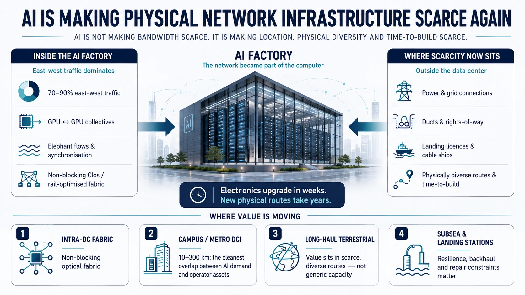
The structural change is real, but it is not the one usually announced. After two decades of software-defined everything, the binding constraints on digital infrastructure have moved back down the stack: to megawatts, ducts, rights-of-way, landing licences, cable ships and the calendar. The most abstract software layer ever built is re-pricing the most physical layers underneath it.

The thesis of this analysis: AI is not making bandwidth scarce — bandwidth per fibre keeps getting cheaper. It is making location, physical diversity and time-to-build scarce again. The strategic asset is no longer capacity; it is capacity in a specific place, on a route nobody else can reproduce within the investment horizon.

1. Auditing the standard AI-and-fibre argument

Most of the widely circulated figures behind the “AI eats fibre” argument are accurate. The problem is not fabrication; it is interpretation — headline numbers detached from the definitions that make them meaningful. Before building a capacity plan or an investment case on top of them, it is worth separating what is measured, what is projected, and what is simply mis-stated.

What holds up

• Content providers account for roughly 75% of used international bandwidth (measured, 2025). TeleGeography has tracked this share since content providers overtook internet backbone operators as the largest users of international capacity in 2017, and projects their capacity requirement growing around ninefold between 2025 and 2035 (projection).
• More than $13bn of new submarine systems are scheduled to enter service between 2025 and 2027 (projection, revised above $14bn in later updates). Subsea cables carry close to 99% of intercontinental data traffic (TeleGeography), which makes this the most concentrated capital cycle in international transport.
• Hyperscale-owned systems of continental scale exist and are funded. Meta’s Waterworth was announced in February 2025 as a system exceeding 50,000 km reaching five continents; Google operates private transatlantic systems and keeps adding Atlantic and Latin American routes; Amazon announced its first wholly owned transatlantic cable between the US East Coast and Cork.
• The optical roadmap from 400G to 800G to 1.6T is real. 800G is in volume deployment inside AI clusters, 1.6T interfaces are entering, and coherent 800ZR interoperability work is active at the OIF while 1600ZR/ZR+ is under development.

What does not survive contact with the definitions

The 75% figure is not a measure of AI traffic. The category counts content providers, cloud providers, AI platforms and neoclouds together. Inside it sit video streaming, search, software distribution, object storage replication, SaaS back-ends and database synchronisation — workloads that predate the current AI cycle by a decade and still dominate the volume. Reading “75% of international capacity” as “75% AI” inflates AI-attributable demand by an unknown but large factor. Nobody publishes the split, and any figure that claims to is an estimate.

The 400G to 3.2T sequence conflates three different measurement planes. The same numbers are used for Ethernet host interfaces, for pluggable optical module capacity and for coherent line rates over distance, and the three do not advance together. What is achievable over 2 km of single-mode fibre inside a campus is not achievable over 2,000 km of amplified line system, and neither is achievable across an ocean without a different generation of submarine line terminal equipment. Coherent 3.2T solutions have been announced with sampling expected around 2027 and commercial availability afterwards. Putting four numbers on one slide compresses several years of physics and supply chain into a visual sequence.

The hollow-core latency arithmetic is usually quoted wrong, even when the conclusion is right. Single-mode silica fibre has a group index near 1.468, which yields a propagation delay of roughly 4.9 microseconds per kilometre — not the 2 microseconds per kilometre that circulates in presentations. Hollow-core fibre with an effective index close to 1.0003 propagates at approximately 3.34 microseconds per kilometre. The saving is about 1.55 microseconds per kilometre, a 31 to 32% reduction, which does match the headline claim; the absolute numbers quoted alongside it frequently do not. On a 100 km metro path that is around 155 microseconds one way and 310 microseconds on the round trip: material for tightly synchronised workloads, irrelevant for almost everything else.

“AI inevitably drives a proportional increase in submarine traffic” is the weakest link in the chain. It is asserted far more often than it is demonstrated, and the mechanics of AI workloads argue partly against it. Section 7 takes that argument apart.

The claim that matters most gets the least attention

The genuinely new fact is a change in which constraint binds. For two decades the limiting factor in transport economics was cost per bit, and the industry solved it repeatedly with better modulation, better digital signal processing, wider bands and denser wavelength grids. In this cycle the limiting factors are grid interconnection queues, transformer lead times, duct availability, right-of-way, landing permits and cable ship capacity. None of those improve on an 18 to 24 month cadence, and none of them can be bought with a faster SerDes — the serialiser/deserialiser circuitry that sets the electrical lane rate feeding each optical module.

2. Inside the AI factory: the network became part of the computer

The first place AI changed network design is the one furthest from any operator’s footprint, and it is where the change is most complete. A conventional data centre carries mostly north-south traffic: hierarchical flows between external users and the servers hosting applications. A large training cluster inverts that. Between 70% and 90% of traffic inside an AI cluster moves east-west, laterally between GPUs, as gradients, weight parameters and optimiser states are exchanged to keep tens of thousands of parallel calculations coherent.

Elephant flows break the statistical assumptions of packet networks

Packet networks are engineered on the assumption of statistical multiplexing. Millions of short, independent, bursty flows — mice flows — average out, which is why oversubscription ratios of 3:1 or higher are normal in enterprise and cloud fabrics. Training backends violate that assumption structurally. They generate elephant flows: massive, sustained transfers that hold interfaces at 100% of nominal capacity for minutes or hours, with synchronisation points where every node transmits simultaneously.

Because distributed training relies on synchronous collective operations, the cluster runs at the speed of its slowest link. Operations such as AllReduce (every node combines its gradients with every other node’s) and AllGather (every node receives the full set) do not complete until the last participant finishes. There is no statistical averaging to hide behind: one congested path, one flapping optic, one mis-tuned queue, and every GPU in the job waits. Vendor and academic modelling puts the sensitivity high — figures circulating in the industry suggest that around 100 microseconds of added jitter on a single link can cost roughly 15% of effective cluster throughput. That specific number should be treated as vendor modelling rather than an independently measured constant, but the direction is not in dispute.

The economics that make this a board-level issue

Network quality inside an AI factory converts directly into cash. Take public GPU rental pricing as the reference: high-end accelerators have been renting in the range of roughly $2 to $4 per GPU-hour across neocloud providers through 2025 and 2026. A 16,000-GPU training cluster therefore represents something on the order of $32,000 to $64,000 per hour of compute — $530 to $1,070 per minute. This is arithmetic on public list prices, not a vendor claim, and it explains the design logic: a fabric that leaves the fleet idle for ten minutes a day destroys more value than the fabric costs.

That is why the objective function changed from availability to job completion time. Traditional network service levels are built around availability percentages and mean time to repair. An AI cluster is dimensioned around Job Completion Time (JCT) — the wall-clock duration of a training run — which is a function of tail latency, jitter, packet loss and congestion behaviour, not of monthly uptime. A fabric with 99.99% availability and poor tail behaviour is a bad fabric.

Non-blocking topologies and rail-optimised design

The architectural answer is a two or three-tier non-blocking Clos fat-tree with rail optimisation. In a rail-optimised design, each GPU port in a server connects to a separate physical network plane, so that traffic between the same GPU index across different nodes — GPU 0 to GPU 0, GPU 1 to GPU 1 — stays confined to its own plane and completes in a minimal number of hops without competing with other rails. Multiplane fabrics extend the same principle across the whole cluster.

The cabling consequence is what makes this a fibre story rather than a switching story. Non-blocking means the aggregate uplink capacity of each tier matches the downlink capacity beneath it, so fibre count scales with GPU count rather than with floor space. Optical connectivity vendors have claimed that AI infrastructure requires at least ten times more fibre connections inside the data centre than previous architectures. That is a commercial claim and should be read as such, but the order of magnitude is consistent with what rail-optimised, non-blocking topologies imply arithmetically.

3. The backend fabric war: InfiniBand, RoCEv2 and Ultra Ethernet

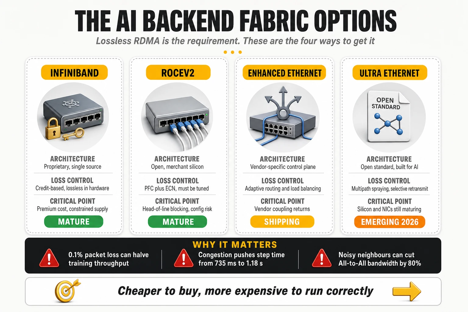
The requirement that defines the AI backend is lossless remote direct memory access. RDMA lets one server write directly into another server’s memory without involving either operating system, which is what makes microsecond-class collective operations possible. RDMA also assumes an almost lossless fabric — and that assumption is where the technology fight sits.

Why 0.1% packet loss costs about half the throughput

InfiniBand solves loss at the hardware layer with credit-based flow control: a sender transmits only when the receiver has advertised buffer credits, so buffers cannot overflow by construction. The result is deterministic behaviour under severe bursts, microsecond-class latency and no retransmission pathology — at the cost of a single-vendor supply chain, premium switching economics and a smaller pool of engineers who can operate it.

RoCEv2 — RDMA over Converged Ethernet version 2 — encapsulates RDMA in standard IP/UDP packets and rides the economics of merchant silicon and the existing Ethernet skill base. The problem is that Ethernet is a best-effort, lossy protocol by design. Classic RoCEv2 implementations retransmit with go-back-N semantics: a single dropped packet forces retransmission of everything sent after it, and because the collective operation is synchronous, the stall propagates to every participant. This is why measurements repeatedly show that a loss rate as low as 0.1% can collapse effective training throughput by around 50%. The non-linearity is the point: a link that would be excellent for enterprise traffic is unusable for a training job.

The tuning burden nobody puts on the datasheet

Making Ethernet effectively lossless requires three mechanisms working in combination, each with its own failure mode:

• Priority Flow Control (PFC): pause frames that stop transmission on a specific traffic class before buffers overflow. Misconfigured, PFC produces head-of-line blocking and, in the worst case, pause storms that propagate congestion backwards across the fabric.
• Explicit Congestion Notification (ECN): switches mark packets as congestion builds, before the buffer overflows. Marking thresholds have to be tuned per buffer architecture and per traffic profile.
• Congestion Notification Packets (CNPs): the receiving network adapter returns notifications so the sender throttles its rate. The control loop latency has to be shorter than the time it takes to fill the buffer, which becomes harder as line rates rise.

The practical implication is an operational one. RoCEv2 is cheaper to buy and considerably more expensive to run correctly. The lower capital cost is real; so is the requirement for a team that understands buffer allocation, marking thresholds and per-class queueing at 800G line rates. Organisations that under-resource that discipline do not get a slightly worse fabric — they get a fabric with intermittent throughput collapses that are hard to attribute.

The noisy neighbour problem in multi-tenant AI fabrics

Standard RoCEv2 configurations do not solve tenant isolation, and that is the unresolved issue for anyone selling GPU capacity rather than consuming it. Published simulation work on large mixture-of-experts training workloads shows uncorrelated background traffic collapsing All-to-All collective bandwidth by more than 80%. In the same body of work, training step time on standard Ethernet degrades from around 735 ms to roughly 1.18 seconds under congestion — a 1.6x penalty — while fabrics with hardware-level adaptive routing, global load balancing and strict plane isolation hold step time near 668 ms. Those figures come from vendor-adjacent simulation rather than independent field measurement, so treat the exact values with caution and the mechanism as well established.

For a GPU-as-a-service provider, this is a product design problem, not a network tuning problem. If tenant B’s traffic can degrade tenant A’s training run by 60%, then per-tenant performance cannot be contracted, and the only honest commercial answer is dedicated planes — which destroys the utilisation economics that made multi-tenancy attractive. Neoclouds that price aggressively without solving isolation are selling a service they cannot guarantee.

Ultra Ethernet: the standards answer, arriving late but arriving

The Ultra Ethernet Consortium released its 1.0 specification in 2025 with a transport designed for AI and HPC rather than retrofitted to them. The relevant departures from classic RoCEv2 are architectural: multipath packet spraying across all available paths instead of per-flow hashing, out-of-order packet delivery with in-order completion semantics, selective retransmission instead of go-back-N, and congestion control designed for incast rather than for wide-area TCP behaviour. The design intent is to remove the head-of-line blocking that makes PFC dangerous at scale.

The three options can be compared honestly on four axes:

• InfiniBand: proprietary and effectively single-source; native lossless behaviour through credit-based flow control; predictable under burst; highest switching cost and a constrained supply chain.
• RoCEv2 on merchant Ethernet silicon: multi-vendor and cost-competitive; lossless only if PFC and ECN are configured and maintained correctly; exposed to head-of-line blocking and to noisy-neighbour effects in multi-tenant deployments.
• Enhanced Ethernet fabrics with adaptive routing and global load balancing: vendor-specific implementations that close most of the gap to InfiniBand while keeping the Ethernet ecosystem; the isolation guarantees are real but come with vendor-coupled control planes.
• Ultra Ethernet: open standard, purpose-built transport, credible multi-vendor roadmap; silicon and NIC availability are still maturing through 2026, so it is a design target for the next build cycle rather than a procurement option for the current one.

Why this matters outside the data centre: the operating standard being set inside AI clusters — zero effective loss, bounded jitter, deterministic behaviour under burst, per-tenant isolation — is the standard those same customers will bring to wide-area procurement when clusters span buildings and campuses. Section 9 returns to what that means for carrier product design.

4. Optics: the adoption cycle compressed, and the power wall arrived

AI has compressed the optical adoption cycle to roughly half its historical length. Enterprise and cloud networks took close to seven years to move from 100G to 400G. The move to 800G consolidated in about three. On the projection side, TrendForce expects global 800G optical transceiver shipments to grow from roughly 24 million units in 2025 to about 63 million in 2026 — a 162% year-on-year increase, and a figure that should be read as a market projection rather than a shipment record.

The demand pull comes from switch silicon, not from the transceiver market itself. A 51.2 Tbps switching ASIC supports 64 ports of 800G in a 2U chassis, and the next silicon generation doubles that again to 102.4 Tbps. Every doubling of switch capacity converts directly into a doubling of module demand, because the ports have to be populated for the silicon to be worth buying.

Optical power is now a first-order line item

Transceiver power has stopped being a rounding error. A fully populated 51.2 Tbps switch running 64 modules at 15W each dissipates around 960W in optics alone, before the ASIC. Scale that to a rail-optimised cluster: a 16,000-GPU deployment with one high-speed port per GPU needs roughly 16,000 GPU-side modules plus the leaf and spine population above them — an installed base plausibly in the 40,000 to 50,000 module range once every tier is counted. At 15W per module that is 600 to 750 kW of optical power alone. This is illustrative arithmetic rather than a vendor figure, but it explains why module power has become a design constraint at the same level as GPU power.

The form factor consolidated on OSFP for thermal reasons. The Octal Small Form-factor Pluggable package offers a larger physical volume and a higher sustained power envelope — roughly 30W against the 14 to 20W typical of QSFP-DD — which is the margin required for coherent and high-order modules. That thermal envelope, not the electrical interface, is why OSFP has displaced QSFP-DD in AI builds.

The mechanical choice that constrains the cooling roadmap

Within OSFP there are two mechanically incompatible designs, and choosing between them commits the facility to a cooling strategy:

• OSFP-IHS (integrated heat sink): finned aluminium or copper heat sink built into the module shell, typically 13 to 21 mm tall. Designed for air-cooled switch chassis where front-to-back fan flow extracts heat from the exposed fins.
• OSFP-RHS (riding heat sink): flat top surface around 9.5 mm thick with no integrated fins, so the heat sink is provided by the host. Required for PCIe network adapters and for cold-plate liquid cooling, where the flat surface couples directly to the plate.

The consequence is a procurement dependency that is easy to miss. A module inventory bought for air-cooled chassis does not transfer to a liquid-cooled retrofit, and a facility planning to move to direct liquid cooling within the asset life of its optics is buying twice. Given that transceiver inventories at cluster scale run into tens of thousands of units, this is a seven-figure decision made by mechanical engineering rather than by network architecture.

LPO and CPO: removing the DSP to buy back watts

For reaches under about 2 km, the industry is pushing Linear Pluggable Optics. LPO removes the digital signal processor from the module and relies on the analogue equalisation of the host switch SerDes. Reported results are a power reduction of roughly 40% — from 15 to 17W down to 8 to 10W per module — and a latency reduction from the order of 100 nanoseconds introduced by DSP and forward error correction processing to under 3 nanoseconds. Applied to the 40,000-module cluster above, a 6W saving per module is around 240 kW recovered, which is real money in a power-constrained facility.

The trade-off is interoperability, and it is not minor. Once equalisation lives in the host, the module and the switch platform have to be qualified as a pair. That reintroduces vendor coupling into the one part of the stack the industry spent fifteen years commoditising, and it makes multi-vendor sparing and second-sourcing considerably harder. Co-packaged optics push further in the same direction, trading serviceability — a failed optic is no longer a field-replaceable unit — for another step down in power per bit. Both are rational answers to a power wall; both narrow supplier choice.

The module classes that matter, by reach

Reach is what separates a data centre component from a carrier-relevant one. The 800G module portfolio maps to distances as follows, with typical power draw:

• SR8 — 50 to 100 m over multimode fibre, 12 to 16W: intra-rack and top-of-rack to leaf connections.
• DR8 — 500 m over single-mode, 14 to 17W: top-of-rack to leaf and spine within a hall.
• 2xFR4 — 2 km over single-mode, 13 to 14.5W: building-to-building within a campus.
• 2xLR4 — 10 km over single-mode, 15 to 18W: campus and short metropolitan routes.
• Coherent ZR — around 80 km, 25 to 28W: metropolitan data centre interconnect (DCI), plugged directly into router ports over a DWDM line system.
• Coherent ZR+ — 120 km and beyond, 27 to 30W: regional interconnect where amplification and dispersion management enter the design.

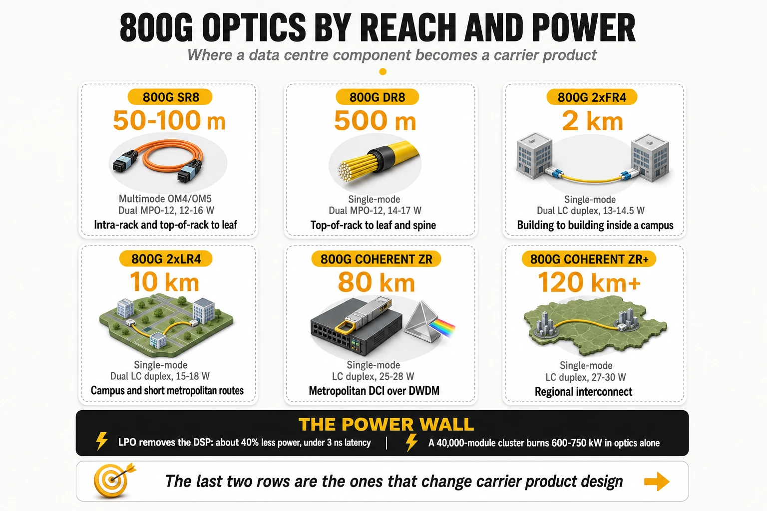
The last two module classes, coherent ZR and ZR+, are the ones that change carrier product design. Coherent pluggables let a customer terminate wavelengths in their own routers and run them as alien wavelengths across someone else’s optical line system. The customer buys spectrum or fibre pairs instead of managed capacity, keeps control of the light, and removes the carrier’s transponder layer from the value chain. That is simultaneously a margin threat and the basis for the highest-value wholesale product available today — a point developed in section 9.

5. When bits per hertz get expensive, you add fibres

Every optical generation buys capacity through some combination of higher baud rate, denser modulation, better DSP, wider bands and improved forward error correction. Each of those levers approaches a physical ceiling, and the closer transmission gets to the nonlinear Shannon limit, the more expensive each additional bit per hertz becomes. C+L band expansion buys spectrum at the cost of amplifier complexity and Raman tilt management. Higher-order modulation buys efficiency at the cost of reach.

Spatial division multiplexing: the unglamorous answer that wins

The alternative is intellectually unsophisticated and economically superior: use more fibres. Modern submarine systems are built around spatial division multiplexing (SDM), which trades capacity per fibre pair for a much higher pair count within the same power budget. Amplifier pump power is shared across more pairs, each pair runs at lower spectral efficiency, and total system capacity and cost per bit both improve. Recent private transatlantic systems are being built with 12 to 24 fibre pairs, against the 6 to 8 pairs typical of the previous generation.

The same logic now applies on land. Multicore fibre packs several independent cores inside the industry-standard 125 micron cladding diameter — four cores multiplying transmission capacity roughly fourfold without increasing cable diameter. Vendor figures presented at OFC 2026 claim reductions of around 70% in cable mass, 75% in connector count and up to 60% in field installation time. Those are manufacturer claims and should be validated against a real duct before being used in a business case, but the direction addresses the actual constraint.

The scarce asset is the duct, not the glass

This is the single most useful reframing available in the current cycle. Glass is manufactured — capacity is being expanded aggressively, and long-term supply agreements between operators and fibre manufacturers have been signed at scale, including one carrier reserving the equivalent of 10% of a major manufacturer’s global fibre output for a two-year period. Manufacturers claim their newest high-density cables allow two to four times more fibre inside the same existing duct.

What is not manufactured is the duct itself, the route it follows, and the legal right to cross the ground above it. A new physically diverse route between two major hubs requires permits, civil works, landing or crossing agreements, power at the intermediate sites, and negotiation with every landowner, municipality, railway and highway authority along the path. That is the asset AI is re-pricing. Fibre count inside an existing duct is a supply chain question; a new duct on a new path is a five-year question.

Hollow-core fibre: from laboratory curiosity to production asset

Anti-resonant hollow-core fibre guides light through an air channel surrounded by a microstructure of silica capillaries with nanometre-scale walls, instead of through doped solid glass. Two properties follow directly from that geometry. First, the latency advantage already quantified: about 3.34 microseconds per kilometre against 4.9 in silica, a 31 to 32% reduction. Second, and strategically more important, the nonlinear coefficient of air is roughly a thousand times lower than that of glass, which allows much higher launch power without nonlinear distortion or cross-phase modulation crosstalk — a direct benefit for dense high-order modulation formats.

The attenuation trajectory is what moved this technology from interesting to investable:

• 2018 (measured): laboratory hollow-core attenuation around 1.3 dB/km, against roughly 0.16 dB/km for standard single-mode fibre. Not a viable transmission medium.
• 2025 (measured, published): 0.091 dB/km reported in the C+L window on a double-nested anti-resonant nodeless fibre, published in Nature by Microsoft’s optical fibre team — below the best solid silica figures for the first time.
• 2026 (reported at OFC, not independently verified): further records claimed in the 0.04 to 0.05 dB/km range on alternative hollow-core structures, which would break through the Rayleigh scattering floor of solid silica.
• Deployment (reported): more than 1,200 km of hollow-core fibre in production metropolitan networks by mid-2026, with a stated roadmap of a further 15,000 km (plan, not installed base).

The ROI case is narrow and specific, and it is worth being precise about where it does not apply. Hollow-core makes sense on latency-sensitive metropolitan and campus interconnect, on financial trading routes, and on links extending a GPU cluster across buildings where every microsecond of round-trip time feeds back into job completion time. It does not make sense in the access network, where propagation delay is a negligible fraction of end-to-end latency. Between those extremes sit the practical obstacles: mode-conversion connectors, hermetic sealing against moisture ingress into the air core, a splicing and field-repair ecosystem that barely exists outside a handful of teams, and amplification schemes that cannot simply reuse the erbium-doped amplifier base. Specialist connectors with insertion losses of 0.1 to 0.3 dB are in production, which is precisely the kind of unglamorous component that decides whether a physics advantage becomes an operational one.

6. The bottleneck moved from bit-rate to time-to-build

Telecommunications engineering advances on an 18 to 24 month cadence; physical execution does not. Civil works, permitting, heavy industrial capacity and grid connection operate on timescales measured in years, and they have become the binding constraint on AI infrastructure. The correct way to read the current cycle is not “how many terabits per second” but “how many quarters until the route exists”.

Power is the hardest constraint, and it is not close

The measured baseline: data centres consumed around 415 TWh of electricity in 2024, roughly 1.5% of global demand, and the International Energy Agency projects that figure more than doubling to approximately 945 TWh by 2030 (projection), with AI-optimised facilities accounting for the majority of the growth. The problem is not generation in aggregate; it is connection in specific places at specific times.

Interconnection queues are the quantified version of that problem. Lawrence Berkeley National Laboratory’s Queued Up analysis has tracked roughly 2,600 GW of generation and storage capacity sitting in US interconnection queues — several times the installed capacity of the entire US grid — with typical wait times from request to commercial operation now measured in years. In Europe’s mature data centre markets (Frankfurt, London, Amsterdam, Paris, Dublin), AI infrastructure developers face waits reported at seven to ten years for large-scale power, and several of those markets have imposed formal restrictions: Amsterdam paused new permits in 2019, Frankfurt has used zoning to constrain new sites, and Dublin has operated under a de facto connection freeze with grid capacity effectively unavailable for new large loads until the late 2020s.

Heavy electrical equipment compounds the delay. Large power transformers — the units required for substations serving hundreds of megawatts — carry lead times reported at three to four years from order, with prices up sharply since 2020 as global demand outran a small number of qualified manufacturers. A data centre shell can be built in one to three years; the transmission reinforcement and substation feeding it can take five to fifteen.

The siting logic inverted, and fibre follows the megawatts

For thirty years, compute was placed where connectivity already existed. Data centres clustered around interconnection hubs, carrier hotels and internet exchange points because that was where the network was. The sequence was: connectivity exists, therefore build here.

The sequence has reversed. AI capacity is now sited where 300 to 500 MW can actually be delivered, which increasingly means locations with no meaningful fibre presence: former industrial sites, areas adjacent to generation assets, secondary markets with spare grid headroom. The new sequence is: power exists, therefore build here, therefore bring fibre urgently. That single inversion is the strongest structural argument for new terrestrial route construction in this cycle — stronger, and far better evidenced, than any claim about submarine traffic growth.

Terrestrial: permits and right-of-way, one jurisdiction at a time

Laying new fibre along secondary roads requires clearing a matrix of local permitting and negotiating public or private right-of-way with agricultural landowners, railway operators, highway authorities and municipalities. Any single objection can delay a build by quarters, and the permitting authority is rarely the same body across the length of the route. This is why incumbent duct and right-of-way portfolios have strategic value that is almost impossible to reproduce: the asset is not the glass, it is the accumulated legal permission to occupy a specific line on a map.

Subsea: the constraint is ships, not capital

Submarine investment above $14bn for 2025 to 2027 has run straight into a physical limit that money cannot resolve quickly. The global fleet of cable laying and repair vessels numbers only a few dozen ships, a large share of them more than twenty years old, and the shipyard capacity to build specialised replacements is thin. A modern cable ship costs in the region of €250m to €300m and carries delivery lead times reported at up to four years — and crewing it requires marine jointing skills that take years to develop and are currently in short supply.

The consequence appears in repair times, not in build times. Mean time to repair a cut cable in contested or heavily regulated waters — the Baltic, the Red Sea — is now reported at more than 40 days, driven as much by permitting and security clearance as by vessel availability. The International Cable Protection Committee (ICPC) records on the order of 150 to 200 cable faults worldwide each year, overwhelmingly from fishing and anchor activity. When a route carries traffic that a training cluster or a production inference service depends on, a 40-day repair window is not a maintenance statistic; it is a business continuity parameter that has to be engineered around with route diversity bought in advance.

The asymmetry, stated plainly

What can be done in weeks to months:

• Upgrading an existing wavelength from 400G to 800G or 1.6T by swapping line cards or coherent pluggables at both ends.
• Lighting additional spectrum on an existing fibre pair, or turning up additional pairs in an existing cable.
• Re-optimising an optical line system, adding amplification, or re-terminating capacity at a different point of presence.

What takes three to fifteen years:

• A new terrestrial route that is genuinely diverse — free of shared risk link groups (SRLGs), the sets of circuits that share a duct, bridge or conduit and therefore fail together.
• A new cable landing station, its landing licence, its marine survey and its backhaul.
• A grid connection and substation of the scale an AI campus requires, plus the transformer to energise it.
• A new cable ship, or the trained marine crew to operate it.

Every strategic conclusion in this analysis follows from that asymmetry. Assets on the first list deflate in value because they can be reproduced quickly by anyone with capital. Assets on the second list appreciate because they cannot.

7. AI does not create one demand curve. It creates four

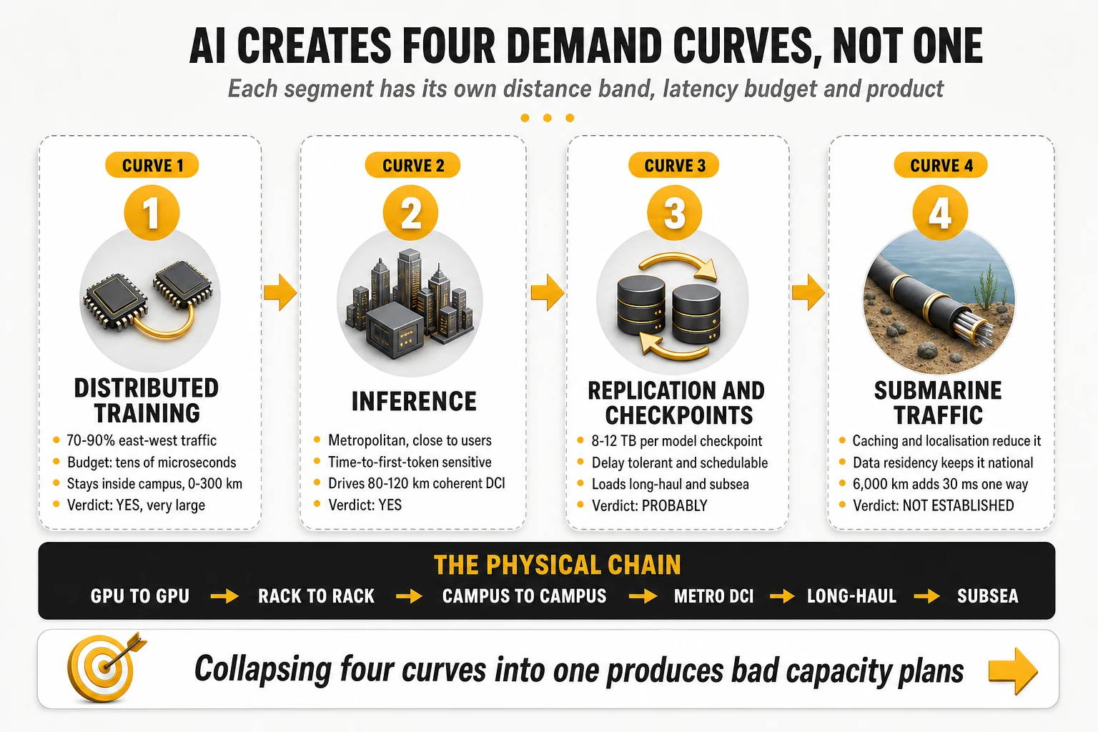
The chain runs GPU to GPU, rack to rack, campus to campus, metro DCI, long-haul, subsea — and the effect of AI is materially different on each segment. Collapsing them into a single “AI needs fibre” statement is what produces bad capacity plans. Each segment has its own driver, its own latency budget and its own tolerance for distance.

Curve 1 — Distributed training: enormous volume, almost no distance

Training traffic is the largest volume and the least geographically mobile, and the reason is arithmetic. Synchronous collective operations complete on budgets measured in tens to hundreds of microseconds. Propagation delay in silica is about 4.9 microseconds per kilometre, so 100 km adds roughly 490 microseconds one way and about 1 millisecond on the round trip — already comparable to or larger than the collective operation itself. A 6,000 km transatlantic path adds around 30 milliseconds one way, three orders of magnitude beyond the synchronisation budget. No amount of bandwidth fixes that; the speed of light continues to decline to cooperate with corporate roadmaps.

What is genuinely expanding is the campus and metropolitan envelope, not the intercontinental one. As single buildings run out of power, training is being distributed across multiple buildings and multiple campuses using asynchronous and pipeline-parallel techniques that tolerate more latency than pure data-parallel synchronisation. Reference architectures now describe linking facilities tens to hundreds of kilometres apart and operating them as one AI factory. That is a real and large new demand for dark fibre and DCI in the 10 to 300 km band. It is not a demand for ocean crossings.

Curve 2 — Inference: metropolitan, asymmetric, latency-sensitive

Inference has the opposite geography. It runs close to users, it is sensitive to time-to-first-token (TTFT) rather than to raw throughput, and it generates traffic patterns that differ from content delivery: more symmetric, frequently upstream-heavy where multimodal inputs are involved, and composed of long-lived sessions rather than short completing flows. Retrieval-augmented generation adds a second effect — each user request triggers multiple machine-to-machine transactions between the model, vector databases and enterprise data sources before a response is produced, so one visible request becomes several invisible ones.

This is the segment where operator assets map most directly onto demand. Metropolitan interconnect at 80 to 120 km, coherent 800ZR and ZR+ wavelengths, edge facility interconnection and low-latency paths between inference sites and enterprise premises are exactly what carriers already own or can extend incrementally. Inference is also the workload most likely to be constrained by data residency rules, which pushes it further towards national and metropolitan infrastructure.

Curve 3 — Replication, checkpointing and disaster recovery: the bulk mover

This is the AI workload that actually loads long-haul and submarine routes, and it is rarely the one being discussed. Training datasets are staged to clusters in advance. Model checkpoints are written during runs and replicated across regions: a trillion-parameter model at 16-bit precision is about 2 TB of parameters alone, and with optimiser states a full checkpoint can reach 8 to 12 TB. Moving 10 TB across a fully utilised 400G wavelength takes roughly 200 seconds of line time — trivial in isolation, substantial when repeated across thousands of runs, regions and retention policies.

The commercially important characteristic of this traffic is that it is delay-tolerant. Bulk replication does not need low latency; it needs large, schedulable, cheap capacity, and it can be moved off-peak. That makes it a fundamentally different product from inference connectivity — capacity on demand, bandwidth calendaring and scheduled bulk transfer, priced per bit — and a poor fit for premium latency-based pricing.

Curve 4 — Submarine: the weakest inference in the chain

Several mechanisms actively work against the assumption that AI converts into proportional submarine traffic growth. Datasets are pre-staged rather than streamed. Trained models are replicated once and served locally. Inference runs close to the user. Outputs are cached. Model distillation and quantisation reduce the size of what has to move. Data residency requirements keep both training corpora and inference logs inside national borders. Each of these localises traffic that would otherwise cross an ocean.

TeleGeography flags precisely this uncertainty: how much AI-driven growth ultimately converts into international long-haul traffic is genuinely unclear, because content localisation, caching, compression and model architecture can all moderate it. The honest position, segment by segment:

• AI drives more fibre inside the data centre: yes, by a large multiple, and this is the best-evidenced claim in the entire narrative.
• AI drives more campus and metropolitan DCI: yes, and this is the segment where operator assets and AI demand overlap most cleanly.
• AI drives more terrestrial long-haul: probably, but mainly as a second-order effect of power-driven siting rather than as direct AI traffic.
• AI drives unbounded submarine growth: not established. Submarine investment is growing for reasons that include AI but are not reducible to it — route diversity, resilience, regional demand and the replacement of end-of-life systems.

8. Who owns the pipes: a shift that started in 2010, not in 2022

The most consequential change in this cycle is ownership, not technology — and the timeline usually given for it is wrong. International infrastructure was historically financed and operated by consortia of carriers. Today four US technology companies design a substantial part of the physical connectivity map. But this did not begin with generative AI. Google participated in the Unity transpacific consortium, which entered service in 2010; content providers became the largest users of international capacity in 2017; by 2025 they accounted for around 75% of used international bandwidth. AI is not causing this shift. It is accelerating a fifteen-year structural change and raising the capital available to complete it.

What the hyperscalers are actually building

• Google: the most active private investor in subsea routes. Privately owned transatlantic capacity connecting the US, the UK and Iberia; new Atlantic systems linking the US East Coast, Bermuda and Portugal; systems in the Indian Ocean and a direct South Pacific route between Chile and Australia. Additional systems in the Americas were announced during 2026 (as reported).
• Meta: private transatlantic systems with high fibre-pair counts landing in northern Spain and Massachusetts, majority ownership in a further transatlantic system, participation in the 2Africa consortium, and Waterworth — a wholly owned system exceeding 50,000 km across five continents with reported investment above $10bn.
• Amazon: its first wholly owned transatlantic cable, a 12 fibre-pair SDM design landing on the Cork coast, marking the transition from capacity buyer to system owner.
• Microsoft: a different strategy — comparatively less private subsea construction, and far more long-term acquisition of terrestrial dark fibre and indefeasible rights of use, combined with the most aggressive hollow-core fibre programme in the industry.

The myth that hyperscalers now fund most new cables

They do not — or at least, it is not demonstrated. TeleGeography has examined this claim specifically and found that content providers do not clearly account for the majority of new submarine builds, although the picture could change if undisclosed private purchases of fibre pairs, spectrum and capacity were included. That caveat is important: the visible part of hyperscaler infrastructure spending is the part with a press release attached, and the invisible part — pairs and spectrum bought from carriers under confidentiality — is precisely the part that matters most to carrier revenue.

Google has been explicit that it runs three models simultaneously: building private cables, participating in consortia, and buying capacity or fibre pairs from carriers, including partnerships with European operators. The relationship is not displacement. It is competitor, customer, supplier and co-investor at the same time — an uncomfortable arrangement for account planning and an accurate description of the market.

The terrestrial deals are the real signal

A cluster of transactions announced between early 2025 and mid-2026 shows where the constraint actually binds (all as publicly reported):

• A US carrier signed a dark fibre supply agreement with Google valued above $1bn in July 2026, with further multi-hundred-million-dollar contracts projected for the remainder of the year. Unlit fibre, not managed capacity.
• A national fibre operator reserved the equivalent of 10% of a major manufacturer’s global fibre output for two years, with a significant share of the deployment consisting of higher-density cable pulled into existing ducts rather than new civil works.
• A second US infrastructure operator signed a long-term supply agreement to secure fibre for a 15,000-mile route expansion through 2030, citing AI-driven pressure on physical supply explicitly.
• Meta signed a fibre and data centre connectivity agreement worth up to $6bn in January 2026, and a GPU vendor and a fibre manufacturer announced a tenfold expansion of US optical connectivity capacity and a more than 50% increase in US fibre production in May 2026.

Read together, these deals say one thing: hyperscalers cannot dig every trench themselves at the speed the market demands, so they are buying the trench from whoever already has it. That converts terrestrial operators with hard-to-replicate assets from suppliers of a commodity into forced co-investment partners. It is a stronger position than most carriers realise, and a weaker one than it looks, because it applies only to the specific routes the buyer cannot build around.

9. What actually changes for carriers: the product mix, not the fibre count

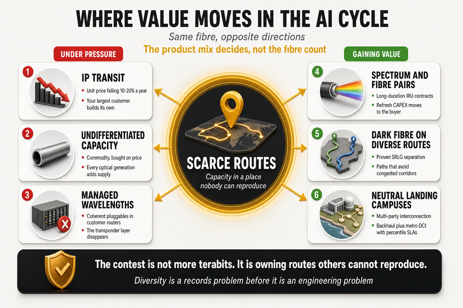
The strategic question for an operator is not how much fibre to build. It is which products survive this cycle. The same physical plant supports products moving in opposite directions in value, and the difference between them is whether the customer is buying bits or buying a position on a map.

Products under structural pressure

• IP transit and undifferentiated lit capacity. Unit prices on major international routes have declined at rates commonly cited in the 10% to 20% range annually (industry estimates, consistent with published price index trends), and each optical generation adds supply to installed fibre without new construction. Selling “100 Gbit/s of transit” to a customer that is building its own backbone is a shrinking business by construction.
• Managed wavelengths where the customer wants control of the light. Coherent pluggables in customer routers remove the operator’s transponder layer from the value chain. Resisting that trend protects a margin line for a few years and loses the account.
• Best-effort enterprise connectivity sold into AI workloads. A product engineered around monthly availability percentages does not meet a requirement expressed in tail latency and loss rate, and the mismatch will be discovered during the customer’s first training run, not during procurement.

Products gaining value

• Optical spectrum services and full fibre pairs under long-duration IRU. Leasing spectral slices lets a hyperscaler inject its own coherent technology and upgrade on its own cycle, while the operator books long-term contracted revenue without carrying the active-equipment refresh CAPEX. This is the single highest-value wholesale product available to a route owner today.
• Dark fibre on scarce routes, particularly paths that avoid congested corridors and provide genuine SRLG separation from the incumbent alternatives.
• Metropolitan and campus DCI engineered to cluster-grade parameters, in the 10 to 300 km band where distributed training and inference actually live.
• Cable landing station backhaul and neutral landing campuses. A landing station evolved into a multi-party neutral facility — where spectrum can be exchanged, local dark fibre loops terminated and metropolitan inference clusters interconnected — converts a single-purpose asset into an interconnection business.
• Contracted physical diversity and restoration. Pre-committed alternative paths with disclosed SRLG separation and hard MTTR commitments, priced as an insurance product rather than bundled free into a capacity sale.

“AI-ready connectivity” has to mean something contractable

Marketing departments have started promising zero jitter and zero packet loss, which is not a commitment any carrier can honour and not what customers are actually asking for. What is contractable, measurable and worth paying for is specific:

• Loss and delay variation expressed as percentiles, not averages — 99.9th percentile one-way delay variation, and loss rates specified with the measurement method and interval attached.
• Disclosed physical path with SRLG separation guarantees, including the commitment not to re-groom the circuit onto a shared duct during maintenance without notification.
• Repair commitments backed by spares and marine agreements, stated as a time to restore with defined exclusions rather than as a best-effort target.
• Telemetry the customer can consume directly, at a granularity that lets them correlate a degraded training step with a network event rather than opening a ticket and waiting.

The prerequisite nobody sells: knowing where the fibre physically runs

Diversity is a records problem before it is an engineering problem. Two circuits sold as redundant that share a duct, a bridge crossing or a building entry are redundant only until an excavator arrives. Many networks assembled through decades of acquisitions have incomplete duct-level records, inconsistent SRLG tagging and no systematic correlation analysis between logical paths and physical infrastructure.

Sophisticated buyers now audit this during procurement. A hyperscaler buying diverse paths asks for physical route data, shared structure disclosure and evidence of separation — and awards the contract to the operator that can produce it. Route knowledge, kept current and auditable, has quietly become a commercial differentiator. It is also the least glamorous investment on any network roadmap, which is why it keeps losing budget arguments to capacity upgrades that generate better slides.

10. The subsea valuation paradox: why 49% margins do not command premium multiples

If physical infrastructure is becoming scarce again, subsea assets should be re-rating. In practice they are not — and understanding why is the best available test of the thesis. European tower carve-outs traded through 2020 and 2021 at multiples in the 25x to 30x EBITDAaL range. Submarine cable businesses, including assets with operating margins near 50%, have changed hands and been marketed at multiples in the 6x to 12x EBITDA range. The gap is not a market error; it reflects five structural differences.

• Recurring technology refresh CAPEX. A tower is a steel structure with a forty-year life and effectively no obsolescence. A submarine system has a design life of around 25 years but requires periodic replacement of submarine line terminal equipment and transponders to stay competitive, which converts a share of EBITDA into maintenance capital rather than free cash flow.
• Price per bit deflation. Tower leases carry inflation-linked escalators. Subsea capacity prices fall year on year, so the same asset sells the same bits for less over time unless volumes grow faster than price declines.
• Marine repair exposure. Fault rates, vessel scarcity and permit-driven repair delays introduce cost and revenue volatility that ground-based passive infrastructure does not carry.
• Customer concentration. A tower portfolio leases to every mobile operator in the market. A subsea route increasingly sells to a handful of hyperscalers, each of which is simultaneously evaluating whether to build its own system on the same path.
• Disintermediation risk. The largest customers are also the most capable potential competitors — a risk profile that has no equivalent in the tower business.

The lesson generalises beyond subsea: a high EBITDA margin is not the same as high free cash flow conversion, and infrastructure investors price the difference precisely. What would genuinely re-rate a route asset is not better margins — it is longer contracted backlog with investment-grade counterparties, IRU and spectrum contracts that transfer the refresh CAPEX to the customer, landing-station real estate with power and interconnection value, and route diversity that the buyer’s alternatives cannot replicate. Those are the same characteristics that make an asset scarce in the sense this analysis has used throughout.

11. The risk nobody is pricing: building too much

Capacity arrives in steps; demand arrives gradually. A new submarine system adds tens or hundreds of terabits per second on the day it enters service. A new terrestrial route adds hundreds or thousands of fibres at once. If several operators build simultaneously against the same exponential demand forecast, the result is a capacity overhang, and the industry has run this experiment before: after the dot-com build-out, only a small fraction of installed long-haul fibre was ever lit, and wholesale prices collapsed for the better part of a decade.

Technology works against the capacity owner in the same way it works for them. Every optical generation extracts more bits from fibre that is already in the ground, which means supply can grow substantially with no construction at all. That is why two apparently contradictory statements are both true and will remain true through this cycle:

• The industry has never needed this much new fibre. Volume demand, fibre counts and connector counts are all at record levels.
• Price per bit will keep falling. Volumes explode while unit economics deflate, which is exactly what happened in every previous transport cycle.

The investment conclusion follows directly. An infrastructure asset is not valuable because it has “AI” in the investor deck or kilometres on the balance sheet. It is valuable if it sits on a route that is scarce, contracted and hard to reproduce within the time-to-build horizon described in section 6. Kilometres in a competitive corridor are inventory. Kilometres on the only diverse path between two hubs are a franchise.

12. 2026 to 2030: five movements, and what would prove them wrong

The following are forecasts, explicitly labelled as such, with the evidence that would falsify each one. A forecast that cannot be disproved is an opinion with a date attached.

• Fibre density inside AI facilities keeps compounding, with 800G in volume, 1.6T ramping, 3.2T arriving late in the period, and a progressive migration from conventional pluggables towards LPO and co-packaged optics as optical power becomes a facility-level constraint. Falsified if module power per bit stops improving and clusters revert to fewer, fatter electrical interconnects.
• Campus and metropolitan interconnect is the fastest-growing segment, because power constraints force AI factories across multiple buildings and sites in the 10 to 300 km band. Falsified if single-site power availability improves faster than cluster scale grows, keeping AI factories inside one campus.
• New long-haul routes get built towards power availability rather than towards traditional telecom hubs, creating fibre demand in corridors with no historical traffic. Falsified if grid reform in mature markets clears interconnection queues fast enough to keep AI capacity in established hubs.
• Hyperscaler vertical integration deepens but stays hybrid, combining private builds, consortium participation, dark fibre purchase and carrier capacity — because none of them can build every trench at market speed. Falsified if a hyperscaler demonstrates it can construct diverse terrestrial routes at scale without carrier assets.
• Value concentrates in ducts, rights-of-way, landing stations and diverse routes, while transit and undifferentiated capacity remain under price pressure. Falsified if permitting and construction timelines collapse, making new routes reproducible in months rather than years.

Signposts worth tracking quarterly

• 1.6T pluggable shipment volumes and LPO share of short-reach ports — the leading indicator for whether the power wall is being solved with optics or with architecture.
• Disclosed dark fibre and spectrum contracts above $500m — the clearest evidence of whether hyperscalers keep buying routes or start building them.
• Announced private subsea systems per year, and the fibre-pair counts within them — pair count is the SDM signal; a flattening pair count would indicate demand normalising.
• Grid interconnection queue reform in the FLAP-D markets — the single policy variable with the largest effect on where AI capacity, and therefore new fibre demand, is located.
• Hollow-core fibre kilometres in production networks and the state of its splicing and repair ecosystem — the difference between a physics result and an operational technology.
• Cable ship orders and deliveries — the most under-reported constraint in international infrastructure, and the one with the longest lag.

13. What to do about it, by position in the value chain

Route and infrastructure owners

• Inventory the assets that cannot be reproduced in five years — ducts, rights-of-way, landing stations, building entries, diverse crossings — and price them separately from capacity. If those assets are currently bundled into a transit product, they are being sold at commodity rates.
• Build the spectrum and fibre-pair product properly, with IRU structures, clear upgrade rights, and terms that transfer the active refresh CAPEX to the buyer. This is the product hyperscalers want and the one with the best cash conversion profile.
• Fix the physical records before the next large tender, because SRLG evidence is now part of procurement, and diversity claims that cannot be substantiated will be discovered during due diligence.
• Convert landing stations into neutral interconnection campuses where feasible; a facility that only backhauls one cable captures a fraction of the value of one that hosts multiple parties, local loops and edge compute.
• Do not build speculative capacity into competitive corridors on the strength of exponential demand slides. Build where the route is scarce and the backlog is contracted.

Data centre and neocloud operators

• Decide the cooling roadmap before buying optics, since the IHS versus RHS choice locks the facility into an air or liquid path across an inventory of tens of thousands of modules.
• Solve tenant isolation before selling multi-tenant GPU capacity, or accept that per-tenant performance cannot be contracted honestly.
• Secure interconnect at the same time as power, not afterwards. A site selected purely on megawatts with a two-year fibre lead time is a stranded asset for the duration of that lead time.

Enterprise and public sector buyers

• Specify AI connectivity in percentiles and physical paths, not in availability percentages. Ask which duct the second circuit runs through, and ask for it in writing.
• Separate the three traffic classes in the requirement — synchronous training, latency-sensitive inference, delay-tolerant bulk replication — and buy a different product for each. Paying premium latency pricing for checkpoint replication is a common and expensive procurement error.

The bottom line

The correct headline is not that AI data centres consume fibre faster than it can be built. It is that AI is making physical network infrastructure scarce again. For twenty years the industry assumed value was migrating upwards through the stack — infrastructure to IP to cloud to software to AI. The most abstract layer of all has turned around and re-priced the most physical ones.

The causal chain is short and difficult to argue with. GPUs need power. Power availability dictates where compute is sited. Distributed compute needs interconnection. Interconnection needs routes. Routes need ducts, permits, rights-of-way, landing licences and, at sea, ships. And none of those scale at the speed of software — which is precisely why they are becoming the scarce asset.

For operators, the conclusion is not that hyperscalers will replace them. It is less comfortable than that: hyperscalers will take the parts of the chain where they do not need a carrier, and they will pay well for the physical parts where they still do. The strategic contest is therefore not about carrying more terabits per second. It is about owning the routes that others cannot reproduce before the demand arrives — and knowing, precisely and provably, where those routes are buried.

---

At TelcoCrux, we help operators, infrastructure owners and investors separate the parts of the AI infrastructure cycle that create durable asset value from the parts that only create capacity. If you need an independent view of which of your physical assets the AI cycle actually re-prices, let’s talk.