Mobile Network Benchmarking: How to measure mobile quality and the engineering actions that move each metric.

The same mobile operator, in the same country and the same quarter, can be ranked first by one benchmark, third by another and merely average by a third. This happens routinely, and it is not a measurement error. Part of the divergence comes from what each house measures — the physical ceiling of the radio link, the experience of the installed base, the service quality of a controlled probe, the outcome of a sequential test suite. The larger part comes from something the industry discusses far less: the chain of decisions that turns millions of raw measurements into a single published number.

That chain contains at least six decision points, and every one of them can change the winner without a single measurement changing. Where the samples were taken and how territories were weighted. How many of those samples are statistically independent. Which threshold separates a successful session from a failed one. Which mathematical function converts megabits per second into a quality score. What weight each service and each data source carries. And what statistical test, if any, was applied before declaring that one operator beat another.

This analysis covers both halves. The first part is methodological and generic: what a benchmark is actually comparing, how measurement architectures differ, how samples and territories are weighted, how technical KPIs become experience scores, how weights are applied, and how statistical confidence is established. The second part applies that framework provider by provider — MedUX, Opensignal, Ookla and nPerf — and then covers application-level testing including generative AI services, the engineering actions that move each indicator, the operators leading each dimension, and a closing protocol for auditing and reproducing any benchmark result.

The thesis: a benchmark result is a measurement plus a model, and the model is rarely published in enough detail to be reproduced. An operator that reads only the ranking is consuming the model’s assumptions as if they were network facts. An operator that can reconstruct the chain — sampling, thresholds, mapping functions, weights, statistics — can tell which part of a gap is its network, which part is the measurement design, and which part is noise.

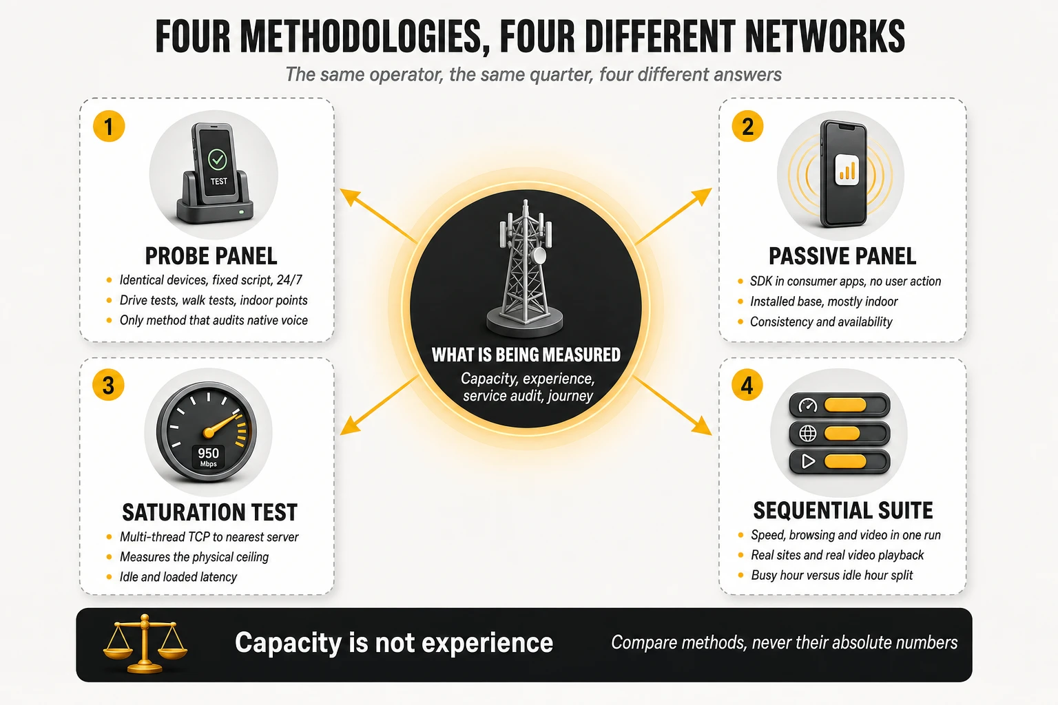
1. What a mobile network benchmark really measures

The object of comparison has to be declared before anything else

Three different objects hide behind the phrase “network quality”, and a benchmark can only measure one of them well at a time.

• Network capability: what the network can deliver to a well-equipped device under favourable conditions. This is what saturation testing with modern handsets on premium tariffs measures, and it is the right object when the question is how much headroom the asset has.
• Delivered experience of the installed base: what the actual subscriber population received, with its real mix of devices, tariffs, locations and hours. This is what passive crowdsourcing measures, and it is the right object when the question is what customers are perceiving.
• Service conformity under controlled conditions: whether defined services meet defined thresholds when every variable except the network is held equal. This is what probe campaigns measure, and it is the right object for engineering audit, regulatory reporting and contractual verification.

The reference methodological framework in Europe is explicit that the object is a designated area, not an abstraction. ETSI TR 103 559 V1.2.1, “Best practices for robust network QoS benchmark testing and scoring”, states that the goal of benchmarking is to determine the best provider for a designated area with respect to the services accessed with a mobile phone, and that results collected in the various areas are individually and collectively weighted and summarised into an overall score. Both halves of that sentence matter: the area is part of the definition, and the summary is a weighted construction rather than an observation.

Four questions every benchmark answers, whether or not it says so

• Which population? Residents, mobile subscribers, data traffic, sessions, or journeys. Weighting by population and weighting by traffic produce different national results from the same raw samples, and only one of them answers a given business question.
• Which places? Roads, dense urban streets, indoor venues, transport hubs, or wherever volunteers happened to be. Place selection is the single largest lever on a benchmark result and the least visible one in the published output.
• Which devices? A normalised flagship fleet measures the network; the installed base measures the service as delivered. Neither is wrong; they are different experiments.
• Which moments? A 24/7 scripted cycle, a busy-hour window, or the moments a user chose to run a test. ETSI advises that measurements be reasonably spread over the different times of day and that busy hours not be deliberately excluded — advice that only has force because the opposite is easy to do.

The governing principles that make a comparison fair

Before any statistics, a benchmark has to survive a set of fairness conditions, and the ETSI report sets them out with unusual directness:

• Fair play. If one operator applies a special QoS construct to the devices used for benchmarking, or a vendor’s firmware recognises benchmark testing and boosts performance, the results no longer reflect customer experience and the networks should not be compared at all.
• Coverage asymmetry handled as a bonus, not a penalty. Operators should never be penalised for providing coverage where others do not; the methodology should measure that difference and reward it, and failures caused by lack of coverage should be included in the scoring rather than excluded as invalid samples. This single rule separates a benchmark that measures networks from one that measures only the overlap between them.
• Technology asymmetry treated the same way. Benchmarking should incorporate the latest technology available on each network, so that early adoption shows up as customer benefit rather than being normalised away.
• Device and server neutrality. Test devices can behave differently on two networks because of antenna placement, band support, firmware or mounting; test servers hosted inside one operator’s network bias latency in its favour. Both have to be chosen so that neither favours a competitor.
• Web page selection rules for browsing tests. At least six different pages, preferably around ten, drawn from public popularity rankings; no ad blockers; no page set dominated by a single CDN; and no sites that users normally reach through a dedicated app rather than a mobile browser. A browsing score built on three pages hosted by one CDN measures that CDN’s footprint, not the network.
• Subscription profile. The highest commercially available profile shows what the network is capable of; budget profiles show what that specific subscriber receives. Mixing the two across operators invalidates the comparison.

The seven-item declaration: the fastest test of any published benchmark

ETSI’s transparency clause lists exactly what every published result should be accompanied by, and it doubles as a checklist for the reader:

1. The scoring model and methodology, including all coefficients, targets and weightings.
2. The underlying KPI values as measured.
3. The number of samples or tests performed for each KPI, in each subcategory.
4. The test methodology, including equipment setup, call sequences, test servers and web pages.
5. The areas and routes used for data collection.
6. The device model and firmware version used.
7. The tariff or data plan used.

Almost no commercial benchmark publishes all seven, and that is not necessarily a scandal — scoring models are commercial assets. But it fixes the correct posture for a reader: the fewer of these items a publication declares, the more the result has to be treated as a vendor’s opinion expressed in decimals, and the less weight it deserves in an investment decision. A quality director who cannot obtain items 1, 3 and 5 for a benchmark that criticises their network has grounds to ask for them before accepting the conclusion.

2. Measurement architectures: probes, crowdsourcing and hybrid models

Two families, four mechanisms

All mobile benchmarking reduces to four acquisition mechanisms, combined in different proportions.

• Controlled active testing: dedicated devices — robotised commercial handsets, vehicle-mounted units, fixed indoor probes — executing a scripted battery of tests on a schedule. Every variable except the network is held constant across the operators compared.
• Crowdsourced active testing: an SDK embedded in consumer applications that runs standardised tests in the background on commercial devices, usually only when a set of activation conditions is met.
• Crowdsourced passive telemetry: continuous observation of radio and connection state — technology in use, signal quality, serving cell, band, standalone or non-standalone attachment, location — without generating traffic.
• User-initiated foreground testing: a test the user chooses to run, typically saturating the link for a bounded interval.

Dimension	Controlled measurement	Crowdsourced measurement
Devices	Equivalent models, firmware and categories	Heterogeneous commercial handsets
Where it measures	Planned routes, locations and service areas	Wherever participants live, work and travel
When it measures	Scheduled cycles across the full day	Whenever activation conditions are met
Comparability between operators	High: one variable isolated by design	Lower: device and tariff mix differ per operator
Spatial and temporal reach	Limited to the campaign plan	Very large, continuous
Diagnostic depth	High: full session traces and radio state	Moderate: aggregated context per sample
Native voice	Measurable with real calls and POLQA scoring	Not measurable; OTT voice only
Indoor representation	Only where indoor points were planned	Naturally indoor-heavy
Dominant bias	Campaign design: routes, targets, device fleet	Panel composition: app mix, devices, demographics
Cost per measurement	High	Very low

Why the hybrid model appeared

The move to hybrid architectures was driven by economics, not by theory. Dedicated measurement robots deliver precision but are expensive to scale: covering a country densely enough to say something about every city, road type and indoor venue requires a fleet and a logistics operation. Providers that started from dedicated hardware have publicly described merging that approach with crowdsourcing and making the measurement software run on commodity devices and operating systems, so the same test logic can execute on a dedicated probe, on a partner’s handset fleet, or inside a consumer application, with the customer choosing the balance between accuracy and data volume.

The result is that the probe-versus-crowdsourcing distinction is now a property of a data set, not of a company. A provider can run a controlled campaign on planned routes, a crowdsourced panel across the same country, fixed probes in homes and venues, and Wi-Fi agents inside apps — and then face the genuinely difficult question of how to express all of it as one number without losing the ability to say which source produced which part of the answer.

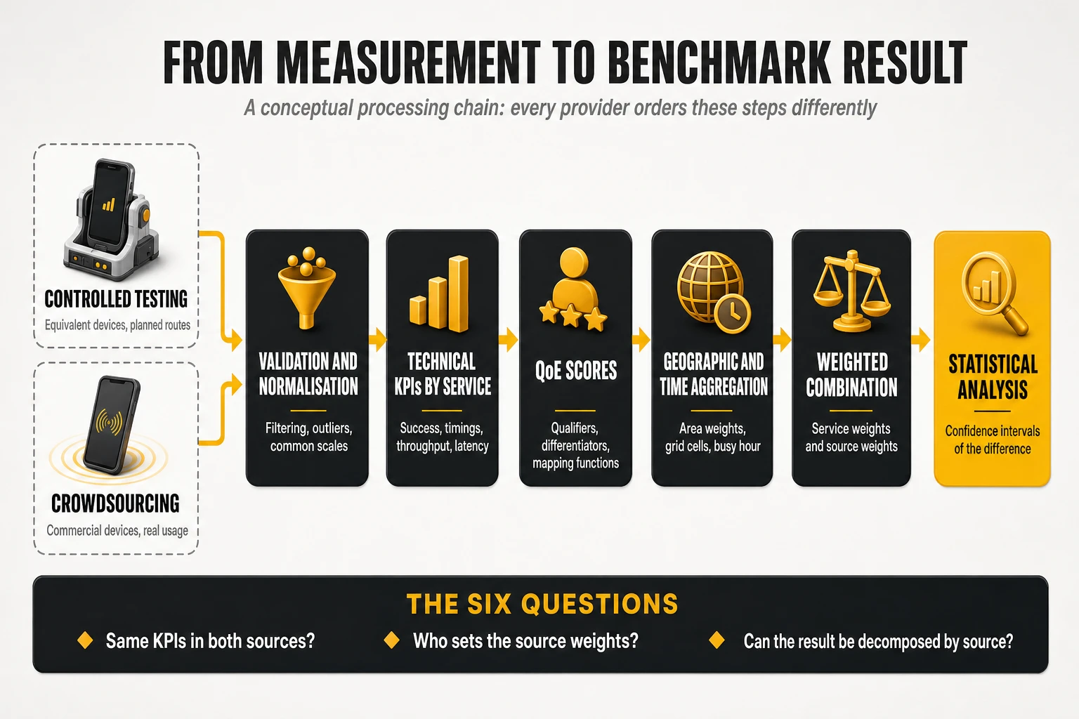
The six questions a multi-source benchmark has to answer

1. Do both sources use the same indicators? If the controlled source measures video startup delay with a real player and the crowdsourced source infers it from throughput samples, the two are not the same KPI and cannot be averaged.
2. Are indicators converted to a common scale before combination? A score built on percentages of samples passing a threshold and a score built on mean opinion scores need a documented transformation before either can enter a joint calculation.
3. Is the geographic distribution normalised before combining? If the controlled campaign is weighted by planned areas and the crowdsourced panel is weighted by where participants happen to be, combining them silently mixes two different target populations.
4. Who sets the weight of each source, and on what basis? This is a methodological decision, not a physical property of the network, and it should be fixed and published before the analysis.
5. What happens when a service exists in only one source? Native voice is the standard case: it can be measured in a controlled campaign and not in a crowdsourced panel. Either the category is excluded from the joint score, or its weight has to be redistributed — and the published number changes meaning depending on which route is chosen.
6. Can the final score be decomposed by source? The most useful question of the six. If an operator scores well in controlled testing and poorly in crowdsourcing, that is a finding, not a contradiction — but only if the architecture allows the two to be read separately.

That last divergence has several possible explanations, and jumping to the flattering one is the most common analytical error in the field. A gap between a strong controlled result and a weaker crowdsourced result may mean that performance available to modern handsets under good conditions is not reaching the real device base. It may equally mean that the two data sets sampled different places, different hours, different tariffs or different device generations. The correct output of a multi-source benchmark is not a single verdict but a decomposition: how much of the gap is network, how much is device mix, how much is where and when each source looked.

Activation conditions: what crowdsourced active testing cannot see

Background tests in consumer applications do not fire at random moments; they fire when a set of conditions is satisfied — typically when the device is connected, idle, not in a call, with the screen off or the application in a particular state, and often only on certain connection types. Those conditions exist for good reasons: they protect the user’s battery, data allowance and foreground performance. They also create a systematic blind spot.

• Moments without connectivity are under-represented in active tests precisely because an active test cannot run when there is no connection. The periods that matter most to a frustrated customer are the periods the active test set is least able to describe.
• Passive telemetry is the corrective. Time-based availability, no-signal rate and technology-residency metrics come from passive observation precisely because they have to include the moments when nothing could be measured actively.
• A benchmark that mixes both must say which metric came from which stream, because an availability figure derived from passive observation and a throughput figure derived from active testing have different denominators and different blind spots.

The same logic applies in reverse to controlled campaigns. A scripted cycle with a fixed wait between tests will under-sample bursty congestion events that last seconds, and a drive route will not observe the lift lobby, the underground car park or the top floor of an office building unless someone planned a walk test there. Neither architecture is blind by accident; both are blind by design, in different directions.

3. Sampling, bias and geographic representativeness

Four quantities that are routinely reported as if they were one

“Billions of measurements” and “millions of devices” are different claims, and the distance between them is where most overstatement in this industry lives. Four quantities need separating:

• Panel devices: terminals potentially available to measure — the installed base of the SDK or the fleet of probes.
• Active devices: terminals that actually contributed data in the measurement window, which is always a fraction of the panel.
• Tests or sessions: individual executions of a test case.
• Measurements or KPI values: the individual numbers produced. One speed test yields a download value, an upload value and a latency value — three measurements, one session, and nothing close to three independent observations.

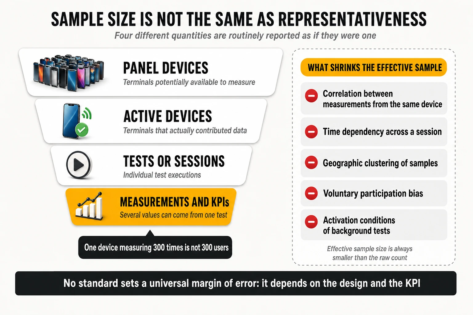
Effective sample size, and why it is always smaller than the headline

Classical confidence formulas assume independent observations. Mobile measurement data violates that assumption in at least five ways:

• Intra-device correlation: three hundred measurements from one handset describe one device, one tariff, one antenna design and one set of habitual locations. They are not three hundred users.
• Within-session dependency: the download, upload and latency values from a single test share the same radio conditions and the same instant of congestion. ETSI’s statistical clause states explicitly that resampling should preserve the correlation between QoS parameters originating from the same service session.
• Temporal dependency: consecutive samples minutes apart in the same cell are closer to one observation of that cell than to two independent draws.
• Spatial clustering: a drive route that passes the same street twenty times, or a panel concentrated in a few neighbourhoods, inflates counts without adding coverage of the target population.
• Voluntary participation: who installs the applications that carry the SDK, and who chooses to run a speed test, are not random selections from the subscriber base.

There is also a resolution problem that no amount of aggregation solves. ETSI illustrates it with ratios: in a collection of 100 calls, one additional dropped call changes the call drop ratio by 1%; with 1,000 calls it changes it by 0.1%. If the real drop ratio sits inside that resolution, the metric cannot describe it reliably no matter how confident the interval looks, and the sample volume has to be increased. The report is explicit that the minimum number of samples and the target confidence interval depend on the purpose of the campaign — which is the correct way to state it, and the reason no universal margin of error should be quoted as if it were a standard.

Good practice in commercial campaigns points the same way. Published benchmarking methodology from the probe-based school states that the confidence level and margin of error are calculated for each deployment and disclosed, that a typical fixed-network benchmark deploys on the order of 45 independent measurement locations per operator, and — the methodologically important part — that repeated measurements over time at the same location are not treated as additional independent locations. That is effective sample size stated plainly: more tests at the same point increase precision about that point, not coverage of the territory.

Where you measure: the area taxonomy

A countrywide benchmark is a stratified design whose strata are geographic, and the reference taxonomy is simple enough to audit:

• Cities, subdivided by size: big cities with high-rise buildings, dense population and most hotspot areas, including main roads, tunnels and bridges; medium cities; and small cities or towns. The subdivision exists because propagation, density and traffic behave differently in each.
• Roads, subdivided by type: highways carrying high traffic between large cities, main roads with intersections and traffic lights, and rural roads connecting smaller settlements. City highways measured inside a city count as city, not road — a detail that changes results when it is applied inconsistently.
• Complementary areas: trains and railways where commuting matters, plus stations, airports, pedestrian zones, parks, stadiums and tourist attractions — the high-density locations where users congregate and where networks most often fail.

ETSI also addresses the awkward case of areas not covered by every operator under test. Limiting a campaign to the areas all networks serve is the simplest option and systematically favours the operator with the smallest footprint; if important parts of the country and population would go untested, either the operator that does not cover them is excluded from the countrywide comparison, or the limitation is carried into the overall scoring. There is no neutral choice here, only a declared one.

How territory is aggregated: the number of passes is not the weight

This is the largest technical gap in most published benchmark commentary. Suppose a campaign collects 10,000 tests in one city, 1,000 in another and 500 in a third. Averaging all 11,500 tests lets the first city define the national result, for no reason other than that the test vehicle spent more time there. Whether that is correct depends entirely on what the benchmark claims to represent: the measurements actually taken, or a target population.

The alternative is explicit weighting, applied at every level of aggregation. A score is computed per territorial unit, units are grouped into categories, each category receives a weight fixed in advance, and the aggregate is built from the category scores rather than from the raw sample pool. ETSI’s worked examples make the arithmetic concrete — and show that the weights are a design choice, not a constant:

• First example set: cities 50%, roads 40%, complementary areas 10%; within cities, big 60% / medium 30% / small 10%; within roads, highways 60% / main 30% / rural 10%; within complementary areas, trains 40% / hotspots 60%.
• Second example set: an 80% / 20% split between cities and outside-cities, with big and medium cities at 45%, towns 20%, hotspots 15%, roads 12.5% and railways 7.5%.
• Both are presented as examples of best practice, not as the standard — and an operator strong on highways and weak in towns will score differently under each, with no change in its network whatsoever.

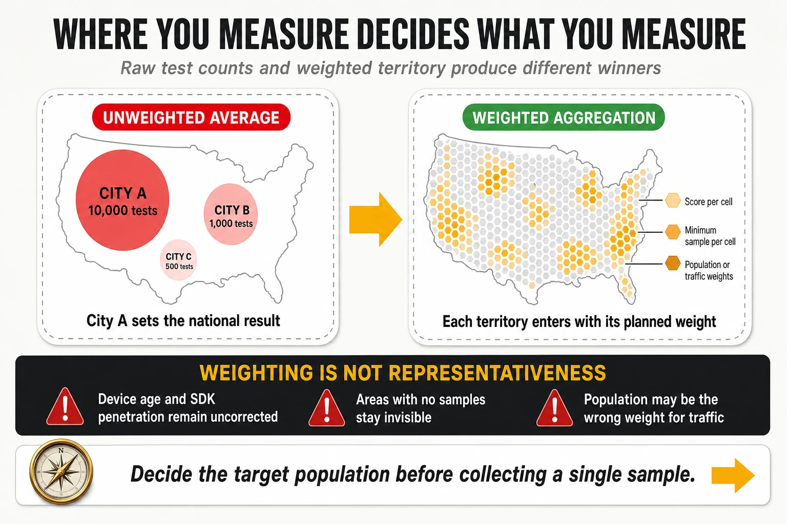
Spatial standardisation of crowdsourced data

Crowdsourced panels need the same correction, applied to a geometry rather than to a route plan. The standard approach is a regular geospatial grid — hexagonal indexing systems such as H3 are common because cell neighbours are equidistant, which rectangular tiles do not give you — with a processing rule set that looks like this:

1. Divide the territory into cells at a chosen resolution.
2. Assign every valid measurement to its cell.
3. Compute a local score per cell.
4. Require a minimum sample — and often a minimum number of distinct devices — before that cell’s score is published or used.
5. Where the minimum is not met, fall back to a larger territorial unit according to predefined rules, rather than dropping the area silently.
6. Aggregate cell scores using weights — population, traffic, or another basis appropriate to the question being asked.

The problem this solves is real: without spatial standardisation, a panel over-weights the areas where the applications carrying the SDK are most installed, which correlates with urbanity, income and device generation. The problem it does not solve is equally real, and overclaiming here is common.

• Population weighting does not correct demographic composition, device age, SDK penetration by handset brand, tariff mix or behavioural differences between participants and non-participants.
• It cannot invent data for cells with no samples. Areas with no participants remain invisible regardless of how carefully the rest is weighted.
• It may be the wrong weight entirely. If the question is about mobile traffic, sessions or mobility rather than residents, weighting by resident population answers a question nobody asked. A commuter corridor carries far more sessions than its residential population implies.

The honest formulation is that geographic weighting converts an uncontrolled sample into a controlled aggregation of an uncontrolled sample. It removes one large bias and leaves several smaller ones in place. That is a substantial improvement and not a claim of statistical representativeness, and the distinction belongs in the methodology note of every report that applies it.

4. From technical KPIs to experience scores

Three aspects per service, always the same three

Whatever the service, scoring frameworks rate the same three aspects, and recognising them makes any scorecard readable:

• Service availability and retainability: did it work at all and did it keep working — success ratio, drop ratio, cut-off ratio.
• Service access time: how long until the service was usable — call setup time, video access time, time to first byte, time to load the first megabyte of a page.
• Quality of the media transfer: how good it was once running — listening quality MOS, video quality and resolution, throughput, freezing time.

Within each aspect, one indicator usually rates average performance and the others rate the tails — the 10th and 90th percentiles, or the share of tests exceeding a defined threshold. That structure is what makes a score sensitive to consistency rather than only to the mean, and it is also where most of the published variation between methodologies lives.

The qualifier: a composite definition of “it worked”

A qualifier is not a single success flag; in current practice it is a composite criterion that a session must satisfy on several dimensions at once before it counts as successful. Published example sets make the construction explicit:

• Telephony: a composite call success criterion combining call setup success ratio, call setup time under 15 seconds, the inverse of the call drop ratio, and the ratio of calls with no two consecutive speech samples below 1.3 MOS. A call that connects, holds and still sounds unusable does not qualify as a success.
• Video streaming: a composite session success criterion combining the video streaming service success ratio with the absence of freezes longer than one second. Only sessions that clear it are then scored for quality aspects — so a network cannot earn quality points on sessions that already failed the user.
• File download: success in accessing and downloading the file, combined with achieving a minimum throughput of around 1,000 kbit/s. Completion alone is not success if it took a form the user would have abandoned.
• Web browsing: success in accessing and downloading at least 1 MB of page content, plus achieving a minimum throughput on that first megabyte. The 1 MB completion criterion exists because modern pages never finish loading in a way that is comparable across sites.
• Interactivity and gaming: the percentage of tests achieving an interactivity score above a floor, computed from two-way latency, latency variation and loss under an application-shaped traffic pattern, following ITU-T G.1051.

The design consequence is the one engineering teams should internalise: the qualifier is where failures are counted, and failures are worth far more score than improvements above the floor. In published example weight sets, composite success criteria carry 55% of a service’s score, while every quality differentiator shares the remaining 45%.

The differentiator: percentiles, and which tail belongs to which KPI

Differentiators separate adequate from excellent, and the percentile chosen must match the direction of the KPI. Getting this backwards is a frequent error in internal dashboards:

• For KPIs where higher is better — throughput, MOS, resolution, interactivity score — the unfavourable tail is the 10th percentile and the favourable tail is the 90th. P10 throughput is the cell-edge and congestion story; P90 is the marketing story.
• For KPIs where lower is better — call setup time, latency, jitter, page load time, video access time — the unfavourable tail is the 90th or 95th percentile and the favourable one is the 10th. Reporting “P10 latency” as a problem indicator inverts the meaning: it describes the best tenth of the samples, not the worst.
• Share-above-threshold indicators complement percentiles: the percentage of download samples faster than 20 Mbps and faster than 100 Mbps, the percentage of upload samples faster than 2 Mbps and 5 Mbps, the ratio of calls with MOS below an unacceptability floor, the percentage of setup times above a long-setup threshold. These are easier to communicate than percentiles and behave identically for optimisation purposes.

Mapping functions: how a megabit becomes a point

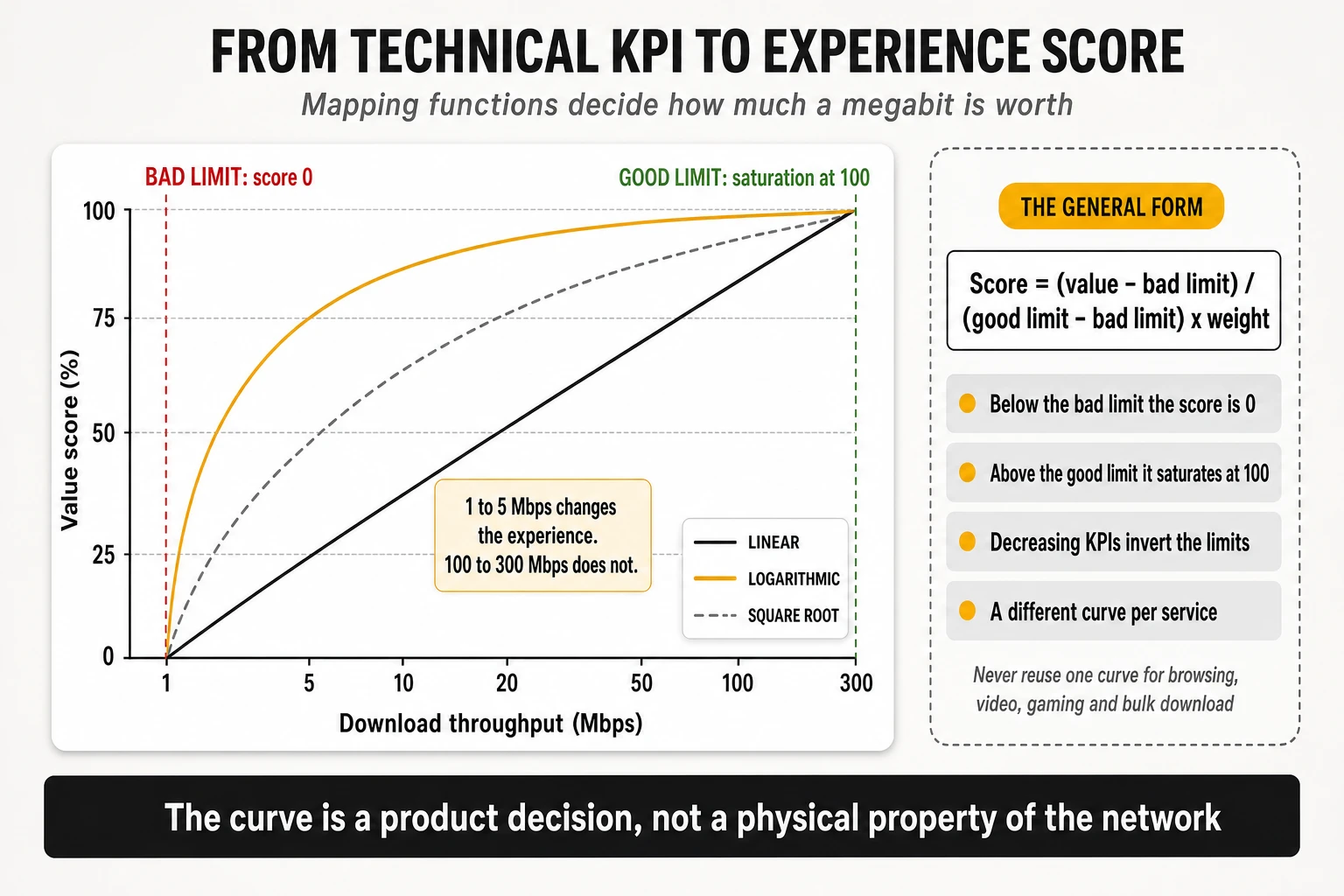
Every scoring framework converts a physical measurement into a bounded value score using two limits and a curve. The published general form is straightforward: each metric has a bad limit, below which customer experience does not meaningfully deteriorate any further, and a good limit, above which it does not meaningfully improve. Between them the score rises from 0% to 100%:

• The linear form: score equals (value − bad limit) divided by (good limit − bad limit), multiplied by the weight, with the result clipped to the 0–100 range. For decreasing KPIs such as latency or setup time, the bad limit is numerically higher than the good limit and the same arithmetic works unchanged.
• Non-linear forms where perception is non-linear: square root, logarithmic and logistic sigmoid functions are the ones in common use. One published example set applies square-root mapping specifically to speech quality, data throughput, average video resolution and file session duration, and linear mapping to everything else.
• A concrete logarithmic transform from the same reference material converts throughput onto a dimensionless 0–1,000 scale before averaging: for downlink, 600 × log10(throughput in Mbit/s + 46) − 1,000; for uplink, 400 × log10(throughput in Mbit/s + 5.6) − 300. The reason for transforming before averaging rather than after is that the mean of a heavily skewed throughput distribution is dominated by its best samples.

The teaching point is the saturation behaviour. Moving a user from 1 Mbps to 5 Mbps changes what they can do; moving them from 100 Mbps to 300 Mbps changes almost nothing for the same service. A scoring model that rewards the second improvement as much as the first is not measuring experience, it is measuring capacity in disguise. And the curve must differ by service: the function appropriate for bulk download is wrong for interactive browsing, and both are wrong for adaptive video, where what matters is holding a stable rate above the resolution ladder’s next rung.

A worked example of the arithmetic

Published example calculations make the mechanism auditable, and reproducing one on a spreadsheet is the fastest way to understand any scorecard. Take a telephony factor with a bad limit of 90% and a good limit of 100% — call setup success ratio — and an observed value of 98%:

• Raw value score: (98 − 90) / (100 − 90) = 0.80, clipped to the 0–100 range as 80.0.
• Weight inside the service: multiply by the factor’s weight within telephony — 25% in one published example set.
• Weight of the service: multiply by telephony’s share of the test score — 40% in that same example.
• Weight of the area: multiply by the weight of the area where the measurement was taken, then sum every factor to obtain the area score, and sum the weighted area scores to obtain the overall result.

Two properties of this arithmetic deserve attention. First, a KPI sitting above its good limit contributes exactly the same as one sitting far above it — which is why benchmark scores compress enormous differences in raw speed. Second, a single factor’s influence on the final number is the product of three or four weights, so a metric that looks important inside its service can be worth a fraction of a point overall. Reading a scorecard without multiplying those weights through is how operators end up optimising indicators that cannot move their published position.

5. Scoring, weighting and benchmark aggregation

Four aggregation layers, each summing to 100%

The canonical structure is a four-layer pyramid: metric, service, area, overall. Metrics are aggregated into a score per service; services are aggregated into telephony and data scores; those are aggregated for the area in which they were collected; and areas are weighted into the overall result. At every level the weights of the children sum to 100% of the parent, which makes the structure auditable even when the coefficients are proprietary.

What this architecture implies is worth stating plainly: there is no such thing as “the” network score. There is a score for a declared set of services, measured in a declared set of areas, weighted by a declared set of coefficients. Change any of the three and the number changes without a single network event.

Two published example weight sets, side by side

The reference report publishes two complete example sets, both labelled as illustrations of practice rather than as a standard. Reading them in parallel shows how much editorial latitude sits inside an apparently technical exercise:

Layer	Example set A	Example set B
Areas	Cities 50%, roads 40%, complementary 10%	Cities 80%, outside cities 20%
Area subdivisions	Big 60% / medium 30% / small 10%; highways 60% / main 30% / rural 10%	Big and medium 45%, towns 20%, hotspots 15%, roads 12.5%, railways 7.5%
Services	Telephony 40%, data 60%	Telephony 36%, data 64%
Data split	Data testing 30%, browsing 25%, video 15%, social and messaging 15%, latency and interactivity 15%	Data testing 45%, video 22.5%, browsing 22.5%, OTT conversational app 5%, eGaming interactivity 5%
Telephony factors	CSSR 25%, drop ratio 25%, MOS 15%, MOS below floor 10%, setup time 15%, long setup ratio 10%	Composite call success 55%, P10 of MOS 22.5%, P90 of setup time 18%, data connectivity during calls 4.5%
Mapping	Linear, with a logarithmic transform for throughput	Linear, with square-root mapping for speech quality, throughput, average video resolution and session duration

Three differences in that table change rankings on their own. Set A gives roads 40% of the national result; set B gives roads 12.5%. Set A scores telephony through six separate factors including average MOS; set B folds four conditions into one composite success criterion and then measures only the bad tail of MOS. Set B also introduces two service categories that did not exist in earlier practice — an OTT conversational app and an interactivity pattern for gaming — each at 5%. An operator optimised for the first model is not optimised for the second.

The second level of weighting: how much each data source counts

In a multi-source benchmark there is a weight above all the others: the share of the final score contributed by each measurement architecture. Conceptually, the global score is the controlled-testing score multiplied by a coefficient, plus the crowdsourced score multiplied by one minus that coefficient. That coefficient is a methodological decision. It is not derived from the network, it cannot be measured, and it is rarely published.

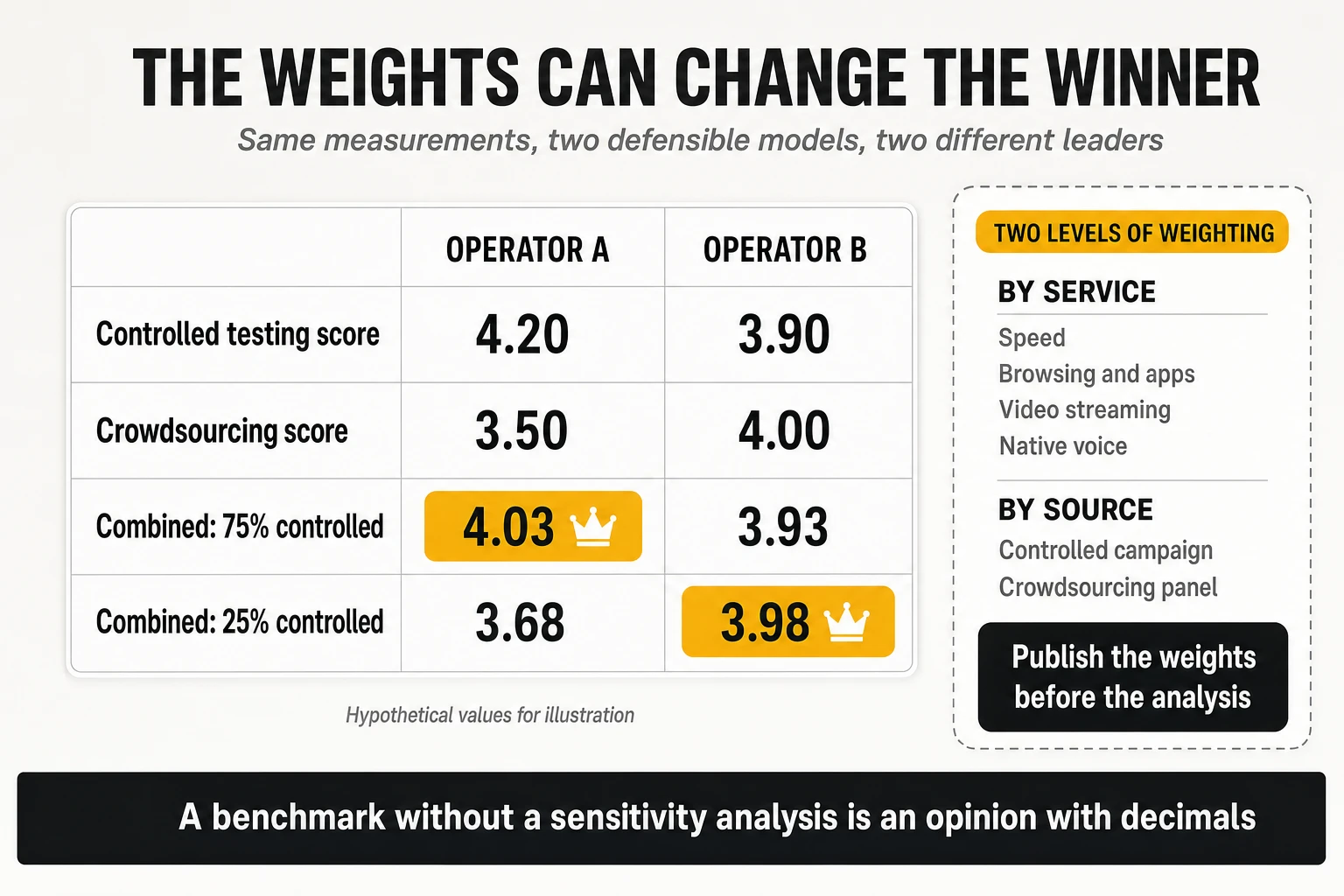
The worked illustration above is hypothetical but entirely realistic. An operator scoring 4.20 in controlled testing and 3.50 in crowdsourcing, against a rival scoring 3.90 and 4.00, leads a model that weights controlled testing at 75% and trails one that weights it at 25%. Neither model is wrong. They define different things as “overall quality”: one leans toward what the network can deliver, the other toward what the installed base received. The error is publishing either one as the answer without stating which question it answers.

Three practical consequences follow:

• Weights must be fixed and justified before the analysis, not tuned after the results are visible. The order of operations is the whole difference between a benchmark and an argument.
• The publication should identify which services and which sources drove the result. “Operator X leads” is far less useful than “Operator X leads because of the voice category in the controlled source, where it holds a 0.4-point advantage worth 0.12 points of the total”.
• A sensitivity analysis should accompany the ranking: how much do the conclusions change when the weights move within a reasonable range? A result that survives a ±25% perturbation of the weights is robust. A result that flips is a statement about the model, not about the networks.

The special case of voice: nominal weight versus effective weight

Native voice can only be measured in the controlled source, which creates an arithmetic trap. If voice carries 30% inside a controlled campaign, and the controlled campaign carries 40% of a combined score, voice’s effective weight in the published number is 12% — not 30%. An operator reading “voice is weighted at 30%” and investing accordingly has misread the model by a factor of two and a half.

The same arithmetic applies in reverse when a technology changes what is measurable. On architectures where native voice over the newest radio technology is not available, a scoring model may assign zero weight to that category and redistribute it to data, video and speed. The resulting score is not comparable with one computed where voice carried a third of the model, and a year-on-year improvement caused by that redistribution is a change of model, not of network.

Four names that are not synonyms

• Overall experience score: the top-level aggregate across all services and areas, on whatever scale the provider uses.
• Reliability or consistency index: a synthetic indicator built from connection, completion and threshold compliance. It is a different construct from the overall score and frequently ranks operators differently.
• Voice experience score: the aggregated score of the voice category, combining accessibility, retainability, setup time and audio quality through weights and mapping functions.
• POLQA MOS: a perceptual estimate of listening quality on a 1-to-5 scale for the audio actually received, defined in ITU-T P.863. It is one input to the voice score, not a synonym for it.

A voice category score of 4.1 on a 0–5 scale and an average POLQA MOS of 4.1 are different statements about different things, and in a published comparison they will rarely coincide. Internal reporting that treats them as interchangeable produces engineering programmes aimed at the wrong indicator.

Weights change between editions, and so do the scores

The reference framework is explicit that test metrics and the relative importance of services change over time, and that the scoring is parameterised precisely so it can keep up. That is methodologically correct and analytically awkward: it means a score from one edition and a score from the next may not be comparable, even from the same provider in the same market.

The practical rule for operators is to treat every published time series as suspect until the methodology note confirms continuity. When a provider adds a service category, changes a threshold, revises a mapping function or redistributes weights, the correct internal response is to re-baseline rather than to celebrate or investigate an apparent jump. The most common cause of an unexplained year-on-year movement in a benchmark score is not the network.

6. Statistical confidence and what “best network” actually means

The two questions a confidence interval answers

A benchmark measures a subset of a population, and two distinct questions follow from that. First, how close is the result derived from the measurements to the experience of the whole population? Second, how repeatable is it — how much would the score move if different measurement points within the same population had been chosen? Both are uncertainty questions, and only the second is addressed by increasing the sample in the same places.

A detail that matters for aggregated scores: different KPIs carry different confidence. A metric that stabilises with few samples and a metric that needs thousands both enter the same weighted sum, and the low-confidence contributors drag down the confidence of the aggregate. When a composite score is published with a tight interval, the relevant question is which of its components actually had enough samples to earn it.

Bootstrap resampling: the method the reference framework actually recommends

Because benchmark scores are built through weighted aggregation of non-normal distributions, closed-form confidence intervals do not apply. The approach documented in the reference framework is empirical resampling, and the pseudo-algorithm is short enough to implement internally:

1. For each measurement contributing to the score, resample from the empirical distribution to generate a bootstrap sample of the same size as the measured set.
2. Recalculate the aggregated QoS parameters and the full score from that bootstrap sample, mapping the result into the score domain.
3. Repeat a large number of times to estimate the distribution of the score.
4. Read the statistical properties off that distribution: confidence intervals, standard deviation, and the spread of plausible scores.

The interpretation is intuitive once stated. With 1,000 individual measurements per aggregated parameter and 10,000 resamplings, the resulting distribution of scores can be read as the outcome of 10,000 hypothetical campaigns run under similar conditions, each producing 1,000 measurements in a different mixture. Two technical cautions travel with it: the resampling must preserve the dependencies between QoS parameters belonging to the same test session, and a Gaussian distribution cannot be assumed for many parameters — throughput in particular — so interval derivation methods that assume normality are inappropriate.

The interval that matters is the interval of the difference

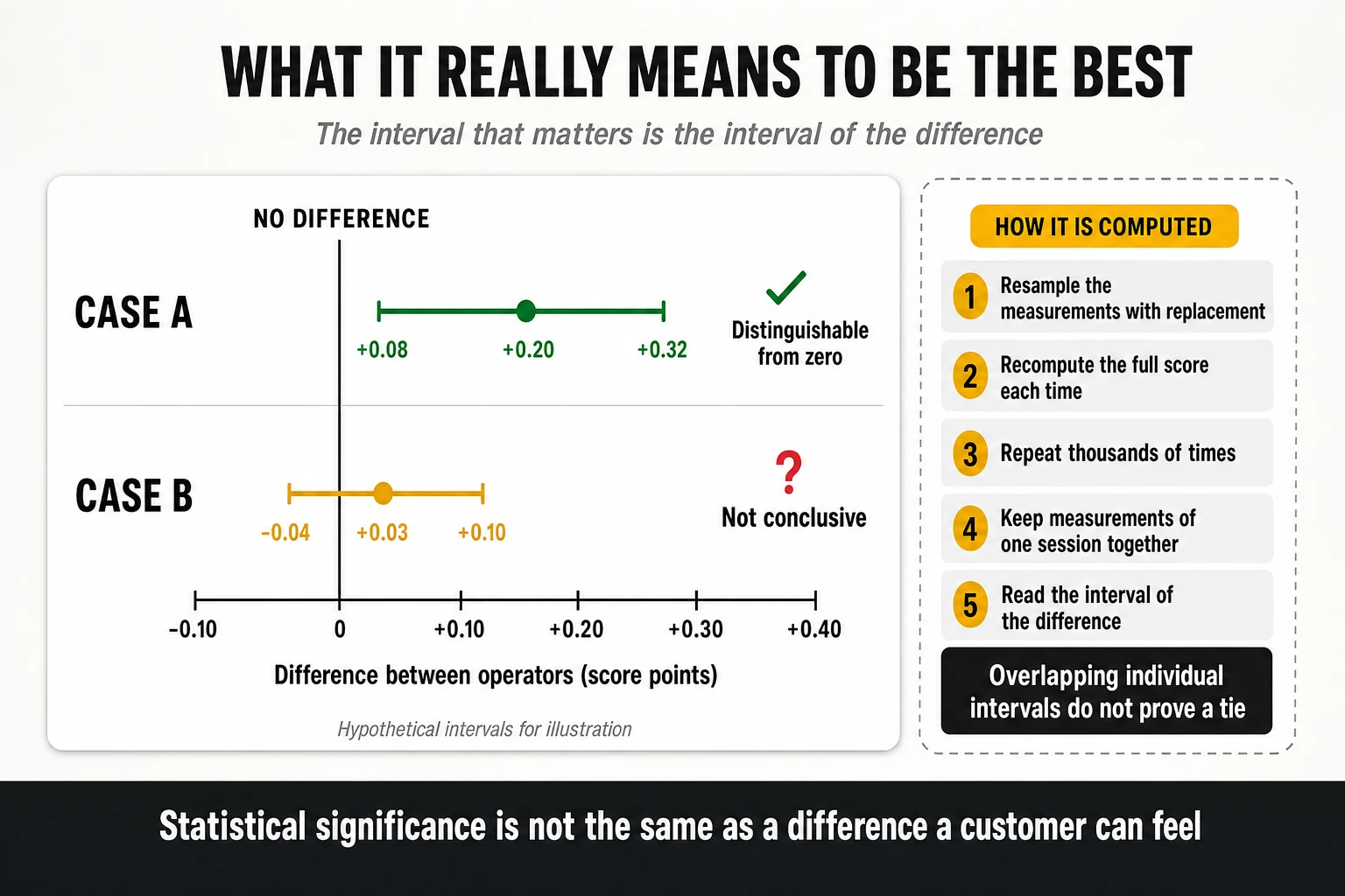
Publishing a confidence interval for each operator is necessary but not sufficient; the question a ranking asks is about the gap between two operators, so the gap is what needs an interval.

Case	Observed difference	95% interval of the difference	Correct conclusion
A	+0.20 points	[+0.08, +0.32]	The difference is distinguishable from zero under this criterion
B	+0.03 points	[−0.04, +0.10]	Not conclusive: the data do not support a claim of superiority

Three refinements separate a careful analysis from a careless one.

• Overlapping individual intervals are not proof of non-significance. Two confidence intervals can overlap while the interval of their difference excludes zero, particularly when measurements are paired. The overlap heuristic is a conservative approximation widely used in award reporting, not a statistical test.
• Measurements taken at the same locations and times are paired, and pairing should be exploited. Comparing operators measured simultaneously at the same points removes a large share of the variance, and a paired analysis will often detect a real difference that an unpaired one cannot.
• Many categories mean many comparisons. A programme that declares winners in eight categories across dozens of markets is performing hundreds of simultaneous tests; without a correction for multiplicity, some “wins” will be noise by construction. Any benchmark that publishes a large award matrix should state how it controls that risk.

Statistical significance is not practical relevance

The reference framework states the limit of its own method with admirable clarity: the significance of a difference between two scores is purely a statistical evaluation and gives no indication of significance in human perception of network performance. With a large enough sample, a difference of 0.02 points becomes statistically detectable and remains perceptually meaningless. The same document declines to recommend a universal significance level, noting that applied levels and comparisons depend on the purpose of the measurement.

A complete leadership claim therefore needs three statements, not one: the size of the difference, the uncertainty of that difference, and an argument that the difference is large enough to matter to a customer or to a business decision. Benchmark publications typically provide the first, sometimes the second and almost never the third — which is exactly where an operator’s own analysis has to take over.

How this shows up in published awards

One widely published implementation of these principles is worth describing because it is visible to everyone. In Opensignal’s awards methodology, when the difference between operators on a given metric is not statistically significant the result is declared a draw and each operator is reported as a joint winner; where confidence intervals are large, the analysis is not reported at all. The practical effect is visible in the published tables: in the 2026 5G awards, a single operator won Video Experience outright among small land-area markets, while twelve operators across four markets shared the equivalent title in the large land-area division (Opensignal 5G Global Awards 2026).

That is a methodological choice with a commercial consequence, and it cuts both ways. It prevents a 0.3 Mbps difference from being marketed as leadership, and it also means an operator can be a “joint winner” alongside eleven others. Neither the discipline nor its side effect is universal: other providers rank by the point estimate and let the reader worry about the interval, which is why cross-provider comparisons of “who won” are comparisons of award rules as much as of networks.

7. MedUX: controlled testing, crowdsourcing and converged QoE scoring

Four data sources, one framework

Describing MedUX as a probe company is now inaccurate: its published framework is explicitly multi-source, and the combination is the methodology. The company’s own materials describe a suite that combines dedicated probes, crowdsourced data, apps and SDKs, and an analytics layer, across mobile, fixed and in-home Wi-Fi (MedUX). Its converged benchmarking framework names four acquisition channels:

• Fixed-network probes: autonomous units connected to the router by Ethernet, running a scheduled test battery across peak and off-peak hours — the Wi-Fi variable deliberately removed.
• Mobile probes: controlled tests on defined routes, locations and service areas, using equivalent devices, configurations, protocols and target servers across every operator compared.
• Wi-Fi crowdsourcing: lightweight agents and SDKs inside commercial applications, running scheduled active tests when device and network conditions are met.
• Mobile crowdsourcing: an SDK running standardised tests, enriched with context — connection type, signal conditions, cellular technology, device model and location.

The services assessed are the same across channels where technically possible: web browsing, data transfer, video streaming, online gaming, social media and cloud access, evaluated by combining technical quality-of-service indicators with service-level quality-of-experience indicators. The company has also stated that future editions of the framework will add assessment areas such as AI readiness and CDN resilience — the first explicit acknowledgment from a benchmarking house that the service mix being measured is about to change.

The controlled leg: what is held constant, and what is not

In the controlled leg, the comparison is engineered rather than inferred. Robotised commercial handsets with retail SIMs execute a fixed script continuously, deployed in three configurations: fixed indoor and outdoor points, vehicle-mounted units for drive testing, and portable units for walk testing in pedestrian areas, transport hubs and indoor venues. Every operator is measured by equivalent hardware running an identical script at the same locations and in the same time windows.

The correct claim for this design is that it removes the largest confounders, not that it isolates the network as the only variable. Identical device models can still behave differently on two networks because of band support, antenna placement, firmware revisions and even mounting position in the vehicle; target-server selection changes the measured path; and the choice of routes decides which parts of each network are examined. Normalisation narrows the set of competing explanations — it does not reduce it to one.

What a real test cycle looks like

Abstract descriptions hide how prescriptive these campaigns are, so it is worth looking at an actual script. A drive-test protocol used in a 2025 mobile benchmarking campaign in a European market ran a fixed loop of 21 scripted tasks per measurement point, repeated continuously:

• Throughput: one multi-thread HTTP download and one multi-thread upload, each opening 20 parallel threads for 10 seconds against servers hosted at a national internet exchange point.
• Voice: three native POLQA-scored calls distributed across the cycle rather than grouped, so voice is sampled under the same range of radio conditions as data.
• Latency: three ICMP ping series toward the three largest social and video platforms, each of 25 packets of 800 bytes at 100 ms intervals — deliberately larger than a minimal echo packet, because small-packet latency flatters a network that queues real payloads.
• Web and social: full page loads through a real browser engine on a search engine, a generative AI service, a news portal and three social platforms — six browsing measurements per cycle.
• Gaming: three latency tests toward the production servers of three different game platforms, using the same packet pattern.
• Cloud and video: a 10 MB single-thread download from a consumer cloud storage service, and a video playback with the resolution ceiling set at 2160p so that time-at-4K is measurable rather than capped by the script.
• Path diagnosis: two traceroutes toward collaboration-service endpoints, which convert every latency result in the cycle into something an engineer can act on.
• Pacing: a 10-second pause between tests, extended to 25 seconds after each call so the radio state following a voice session does not contaminate the next data measurement.

Two design decisions in that script deserve attention. The test targets are the platforms customers actually use rather than neutral test servers, so the result includes the operator’s peering and CDN position by construction. And the pacing rules exist to stop one measurement polluting the next — a control no crowdsourced panel can apply, and the reason probe results are reproducible while crowdsourced results are only statistically stable.

The crowdsourced leg: two measurement families, two latency definitions

The SDK-based data set running alongside the probe fleet uses a different architecture, and understanding it prevents a common misreading. Measurements fall into two families executed in sequence:

• The UDP leg: a burst of 100 packets of 44 bytes toward a regional measurement server using the TWAMP protocol defined in RFC 5357. Latency is reported as the minimum observed value expressed one-way — half of the round trip. Jitter is the average of the absolute delay differences between consecutive packet pairs, and packet loss is the ratio of unconfirmed packets to packets sent.
• The CDN leg: executed against the nearest point of presence of a global content delivery network, in a fixed order — server selection, latency, downlink, uplink. It reports time-to-first-byte as the elapsed time from the GET request to the 200 OK response, latency and jitter from a short ICMP series of 10 packets of 64 bytes, and throughput from multiple parallel HTTP streams using files of different sizes.

The practical consequence is a trap for anyone comparing figures: the same data set can report two latency values differing by a factor of two, because one follows a one-way convention and the other a round trip. Regional measurement servers add a second complication — a probe in one continent measuring against a server in another is not measuring a comparable path, which is why these architectures progressively migrate to per-country servers.

Sample design, confidence and what gets disclosed

• Normalisation: equivalent device models, firmware and categories, and commercial retail tariffs with no engineering SIMs, no prioritisation and no test-server whitelisting — so throttling and fair-usage policies form part of the measured result rather than being bypassed by it.
• Stratification: routes and static points allocated in advance across dense urban, urban, suburban and rural strata and across indoor and outdoor environments, in proportions fixed by the campaign design rather than by where users happen to be.
• Per-deployment statistics: the published framework states that the confidence level and margin of error are calculated for each deployment and disclosed, rather than asserted as a constant. For fixed benchmarks it cites a typical design of around 45 independent measurement locations per operator.
• Independence discipline: repeated measurements over time at the same location are explicitly not counted as additional independent locations — the single most important sentence in any crowdsourcing or probe methodology note.
• Per-publication declaration: each award or report specifies the sources used, the networks and services covered, the measurement period, the scoring configuration and the supporting evidence.

The residual bias is structural and worth naming: the route is the result. A drive test measures the network along the roads someone chose to drive, and a route plan that over-weights motorways flatters operators with strong macro coverage along transport corridors while under-representing indoor performance, where most mobile data is consumed. That is why the area taxonomy and weights of section 3 are not an academic detail — they are the difference between two legitimate campaigns producing opposite rankings.

Application-layer KPIs, service by service

• Web browsing: a real browser engine loads a real site; the suite reports DNS lookup time, time-to-first-byte per resource and total load time until every element has rendered. DNS is broken out separately because it can account for a large share of perceived page load time on mobile.
• Video streaming: startup delay (player loading plus time to first frame), average resolution sustained, percentage of session time at maximum resolution, number of stalls and total stall duration excluding initial buffering. Reporting time-at-full-resolution separately from stalls matters: a stall-free session that never leaves 480p is still a poor session.
• Gaming: latency, jitter and packet loss toward the production servers of real multiplayer titles — a measurement of the operator’s routing and peering toward game platforms, not only of the radio link.
• Social media: the same browsing instrumentation applied to social platforms, where client-side rendering makes session duration behave differently from news or portal sites.
• Cloud transfer: single-thread download of a fixed-size file from a consumer cloud service, reporting download time and the P10/P90 of the observed rate. Single-thread behaviour exposes congestion and loss that a 20-thread test masks.
• Traceroute: hop count and per-hop delay toward application endpoints, which turns a latency result into a diagnosis.

Native voice: the capability no crowdsourced panel has

This remains the single largest methodological differentiator in the market: controlled campaigns place real telephone calls, and crowdsourced panels do not. A pair of probes calls over the operator’s native telephony service — VoLTE on 4G, VoNR on 5G Standalone, or circuit-switched fallback where it still exists — transmits a reference audio sample and scores the decoded audio with POLQA (ITU-T P.863), or with PESQ (ITU-T P.862) in legacy configurations, producing a mean opinion score on a 1-to-5 scale. The KPI set follows the ETSI TS 102 250 definitions:

• Call setup success ratio: attempts reaching the alerting phase without being blocked in IMS signalling — the accessibility metric.
• Call setup time: from dialling to ring-back, dominated by SIP handling, radio bearer assignment and, where native 5G voice is absent, by the fallback procedure. Note that trigger points taken at the user interface differ in time from signalling-layer trigger points, which is why two providers can publish different setup times for the same network.
• Call drop ratio: established calls terminated by the network — the retainability metric, most sensitive to handover parameterisation and coverage holes.
• Fallback and return time: the delay when a 5G-attached device moves to 4G to place a call, and the time to return afterwards. Invisible in crowdsourced data, highly visible to customers.
• MOS and sub-threshold MOS share: the average score plus the percentage of calls below an unacceptability floor. Scoring frameworks also use the ratio of calls containing consecutive speech samples below a very low MOS as an explicit unsustainability indicator.

4G, 5G NSA and 5G SA: what the split does and does not mean

Because the probe reads modem-level state rather than the handset status bar, results can be separated by actual radio access technology and core attachment, logging RRC state, serving cell, band and network service state with every test. Scoring models are then configured per architecture. Three cautions apply to the way that split is usually reported:

• A non-standalone architecture does not mean the customer has no native telephony. VoNR requires standalone, but VoLTE continues to carry voice on the LTE layer, and it can be excellent. A model that assigns zero weight to voice when scoring 5G NSA is making a scoring decision about what is attributable to 5G — not a statement that those customers lack a voice service.
• A weight redistribution is not an experience improvement. If voice weight is reallocated to data and speed under one architecture, the resulting score moves for modelling reasons. Comparing it with a score computed under a different weight allocation measures the model.
• Technology attribution needs its denominator stated. A score computed only on 5G samples describes performance conditional on being on 5G, which is a different statement from the experience of a 5G customer across a day — and the gap between them is exactly the share of time spent on other technologies.

Converged scoring: qualifiers, differentiators and source visibility

The scoring architecture follows the three-stage pattern described in sections 4 and 5: each test is checked against a qualifier — completed without errors and within defined thresholds — then scored on differentiator KPIs that reward performance above the floor; KPIs are combined into a score per service category; and service scores are weighted into a global figure. A scorecard model documented for a 2025 campaign distributed service weights as data and OTT applications 30.5%, voice 30%, video streaming 22%, value for speed 13% and accessibility 4.5%, with qualifier thresholds such as a browsing session under 13 seconds, DNS under 70 ms, TTFB under 400 ms, video startup under 5 seconds, gaming packet loss under 3% with round-trip time under 100 ms, and a call setup success ratio above 90%.

The distinguishing claim of the converged framework is traceability rather than a particular formula: the published position is that the scoring framework preserves visibility into every measurement source, and that each publication declares which sources contributed. That is the right answer to the sixth question of section 2 — whether a result can be decomposed — and it is the property an operator should insist on contractually, because without it a multi-source score cannot be acted upon.

Strengths, limits and residual bias

• Strengths: reproducibility in the controlled leg, device and tariff normalisation, application-layer measurement with real clients, diagnostic traceability — a bad result arrives with the DNS time, the TTFB, the hop path and the radio state that caused it — the only objective audit of native voice at scale, and a scale extension through crowdsourcing that pure probe campaigns cannot reach.
• Limits: controlled sample volumes orders of magnitude below crowdsourcing, cost per measurement, geographic coverage restricted to planned routes and points, a device fleet deliberately better than the average handset, and a combination step whose weights are a modelling decision.
• Residual bias: route and point selection, choice of test targets, the proportion assigned to each source, and — in the crowdsourced leg — the composition of the application panel and the activation conditions under which background tests fire.

8. Opensignal: passive crowdsourcing at panel scale

How the data is captured

Opensignal occupies the opposite end of the methodological spectrum: it measures the network as the installed base experiences it, on the devices people own, in the places they go. Data comes from an SDK embedded in thousands of consumer applications across Android and iOS, measuring automatically in the background while the user goes about a normal day. The user never initiates a test and never sees one. The 2026 Global Awards were built on billions of measurements collected directly from user devices over the 180 days of the second half of 2025, covering 266 operators across 82 markets (Opensignal Global Awards 2026).

The capture combines two streams, and the distinction governs what each metric can mean. The passive stream logs radio and connection state continuously — technology in use, signal quality indicators such as RSRP, RSRQ and SINR, band, serving cell, standalone or non-standalone attachment, approximate location — without generating traffic. The active stream runs short automated transactions at randomised intervals: throughput tests, latency probes, video playback samples and measurements toward gaming endpoints. Availability and technology-residency metrics come from the passive stream because they must include the moments when no active test could run; throughput and application metrics come from the active stream.

Test types and cadence

• Speed tests: larger, time-boxed transfers — a few hundred megabytes on 4G, larger files on 5G, capped at around ten seconds — run at low frequency, returning download speed, upload speed and TCP ping latency. This is the closest equivalent to a capacity test in the catalogue.
• Throughput tests: small automated transfers, on the order of a few megabytes down and about a megabyte up, run roughly daily, returning end-user throughput and time-to-first-byte under load. These reflect ordinary application behaviour rather than saturating the link.
• Server response tests: UDP packet bursts run approximately hourly, returning one-way latency, packet loss and jitter — UDP because it exposes transport behaviour without TCP’s retransmission masking.
• ICMP ping: small echo bursts, also roughly hourly, giving a second independent latency and loss series.

Two structural properties follow from this design. Tests terminate in major content delivery networks and public clouds rather than operator-hosted servers, so the figure describes the end-to-end path a real application traverses and cannot isolate a network segment: it will not say whether a problem lives in the radio, the backhaul or the interconnect. And the cadence applies only to the fraction of time the SDK is active and its activation conditions are met, which is why the panel size and the measurement count are not the same thing.

Aggregation and bias control

• One device, one vote: measurements from a single device within an observation period and geographic area are averaged internally before entering the operator aggregate, so a hyperactive user or a device parked in one location cannot move a national average. This is the practical implementation of effective sample size discussed in section 3.
• Outlier filtering: anomalous and extreme values are removed by statistical filters before aggregation.
• Classification and stratification: results are classified by operator, technology and geolocation and aggregated to country, region and city level, preserving the technology mix each operator’s users actually experienced rather than normalising it away.
• Observation windows: published reports typically use a 90-day period, with shorter windows of around 30 days for rapid analyses and 180 days for the global award cycles. Longer windows stabilise the sample; shorter ones detect change faster.
• Independence from operators: measurements are not commissioned, scheduled or supplied by operators, and controlled test campaigns are not accepted into the data set — the mirror image of the probe school’s logic, and the reason the two data sets should never be merged naively.

What this methodology actually represents

It measures the aggregate experience of a subscriber base, weighted by where and when those subscribers live their lives. Because most mobile data is consumed indoors, the data set is heavily indoor-weighted, which makes it unusually good at detecting dead zones and in-building degradation and unusually poor at describing the network’s physical ceiling. An operator with excellent outdoor urban capacity and weak indoor penetration will look worse here than in any other methodology — and its customers will agree.

The speed family: five metrics that are not interchangeable

• Download and Upload Speed Experience (Mbps): the typical everyday speeds users experience across an operator’s mobile data networks. This is an average across the technologies users were actually connected to, so it embeds availability as well as speed.
• 5G Download and 5G Upload Speed (Mbps): averages observed only while an active 5G connection was in use — performance conditional on 5G, isolating the radio and core from the technology mix.
• Download Speed Experience — 5G Users (Mbps): the average experienced by users with a 5G device and subscription, factoring in 2G, 3G, 4G and 5G speeds together with the availability of each. This is the metric that punishes an operator whose 5G is fast but rarely available: the customer paid for 5G and spent most of the time on 4G.
• 4G and 3G Download Speed (Mbps): per-technology averages, useful for diagnosing whether a weak overall result comes from the 4G layer rather than the 5G layer.

Reading the wrong member of that family is one of the most frequent errors in competitive analysis. A press release citing 5G speed and an internal dashboard citing speed experience for 5G users are describing the same network with a difference that can exceed a factor of two, and the difference is availability, not radio performance.

Consistent Quality: the threshold metric and how it is computed

Consistent Quality is the most operationally useful metric in the crowdsourced catalogue, because it replaces averages with pass/fail thresholds. It measures how often the network was sufficient to support common application requirements, computed as the proportion of tests passing every threshold, multiplied by the test success ratio — the share of attempted tests that completed at all. A test passes only if all component metrics pass; one failure fails the whole test. Two threshold sets are published:

• Excellent Consistent Quality, built on the requirements of demanding services such as HD and live video and cloud gaming: download ≥ 5 Mbps, upload ≥ 1.5 Mbps, latency < 50 ms, jitter < 12 ms, packet discard < 1%, time to first byte < 800 ms.
• Core Consistent Quality, built on common but less demanding use cases — SD video, browsing, email, photo sharing: download ≥ 1.5 Mbps, upload ≥ 500 kbps, latency < 100 ms, jitter < 20 ms, packet discard < 4%, time to first byte < 1.2 s.

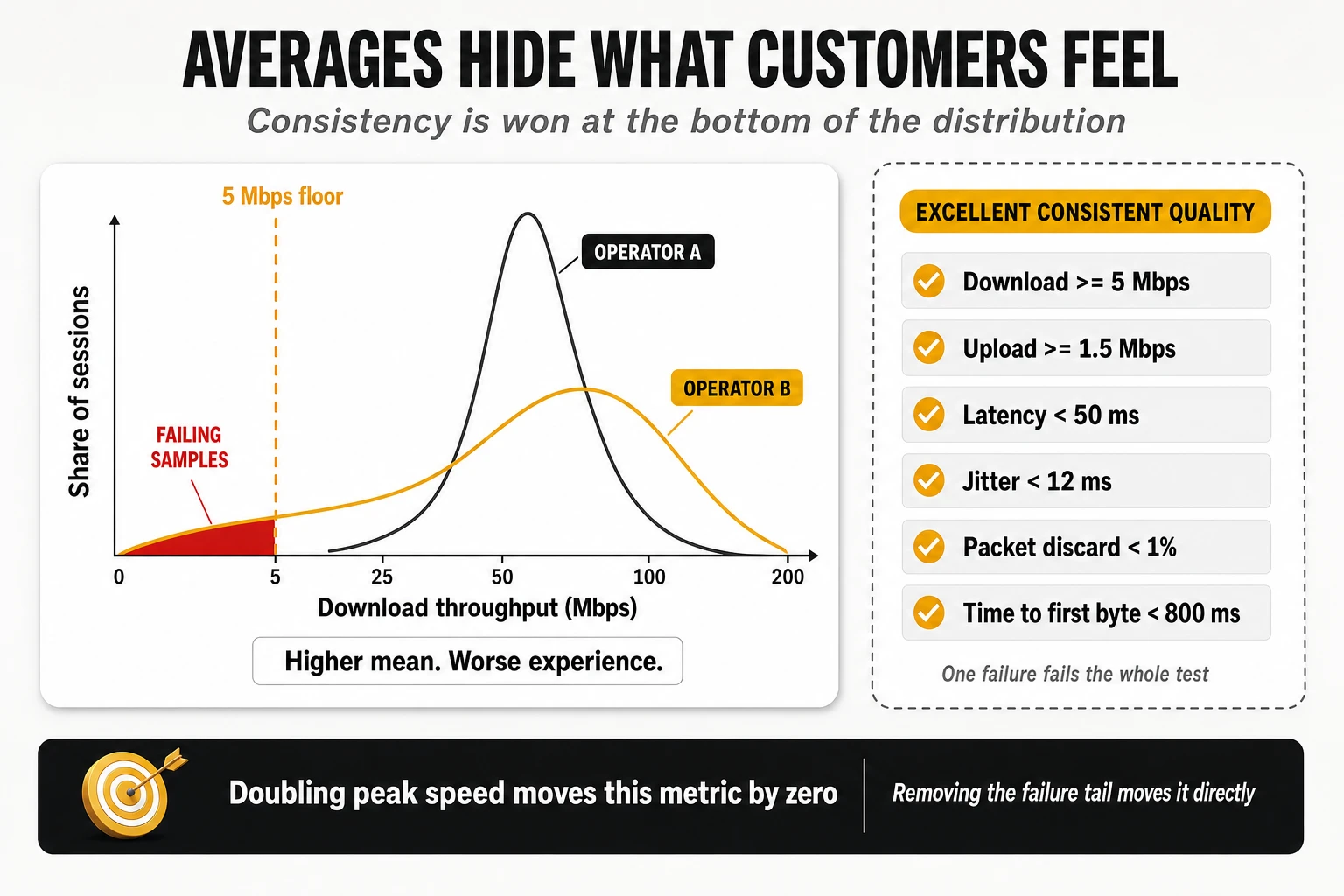
The engineering implication is why this metric deserves priority over headline speed. Doubling peak throughput from 300 to 600 Mbps moves Consistent Quality by exactly zero, because both values clear every threshold. Removing the 4% of samples sitting below 5 Mbps or above 50 ms moves it directly. It is a metric about the bottom of the distribution, and the bottom of the distribution is what generates complaints.

Reliability Experience: connect, complete, suffice

Reliability Experience is scored from 100 to 1000 and answers three sequential questions rather than one:

• Connectivity: the proportion of time users can successfully connect to a mobile network, and the proportion of time the network is available and the device can reach the internet.
• Task completion: whether tasks initiated by the device actually complete, measured with an active UDP test toward a test server, on a 0–100% scale.
• Sufficiency: the probability that a task executes well enough — the percentage of tests passing all required thresholds, where failing any one threshold sets sufficiency for that session to zero. In the mobile metric the thresholds are download > 1.5 Mbps, upload > 0.5 Mbps, latency < 100 ms, jitter < 20 ms, packet discard < 4% and time to first byte < 1.2 s.

Published interpretation bands, derived from user research, give the scale meaning: 600 and above corresponds to users who describe their connection as highly reliable; 400 to 600 is the range where perception is mixed and is influenced by price, competition and expectations as much as by the network; below 400 users describe the service as unreliable. The metric explicitly excludes standard voice calls carried by the operator’s own telephony service — it covers data connectivity and OTT applications only, which is the single most important caveat attached to an award named “reliability”.

Application experience: video, live video, games and OTT voice

• Video Experience (0–100): quantifies adaptive video streamed to mobile devices by measuring real-world streams from the largest content providers, at resolutions from 144p to 2160p. The model uses a mean-opinion-score approach derived from ITU studies — the reference work being ITU-T P.1203 — evaluating time to start playback, picture quality including the resolution achieved, time spent playing at each resolution, and time spent re-buffering.
• Live Video Experience (0–100): the same approach extended with live playback offset — how far behind real time the stream runs — which is what decides whether a live sports feed is usable.
• Games Experience (0–100): measures real-time multiplayer gaming as affected by latency, packet loss and jitter, using end-to-end measurement from user devices to endpoints hosting real games, calibrated against research on how players perceive those conditions across genres.
• Voice App Experience (0–100): measures over-the-top voice services — messaging and calling applications — using a model derived from the ITU approach to overall call quality plus calibrated technical parameters. It does not place, and does not measure, a native telephone call.

These are model outputs, not direct observations, and that has an operational implication. An ITU-derived score computed from real streams and a stall-and-resolution measurement from a scripted player are different constructs even when both are printed on a 0–100 scale. Comparing them across providers is comparing models; comparing either one against itself over time is legitimate as long as the model has not been revised.

Coverage, availability, reach and time on network

This family is the most frequently misread in the industry, and Opensignal is explicit that its availability metrics are not measures of a network’s geographical extent:

• Coverage Experience (0–10): the extent of the network in the places people live, work and travel — a geographic measure of populated areas weighted by where users actually go, rather than by land area or population density alone.
• Availability: the proportion of time users have a connection on a usable network. Time-based, not location-based.
• Time on Network and Time on 4G/5G: the proportion of time users had a 3G, 4G or 5G connection, and the proportion with 4G or 5G specifically. The latter is the variant used in global award reporting.
• 5G Availability and Time on 5G: the proportion of time users with a 5G device and subscription had or used an active 5G connection. An operator can hold high theoretical population coverage and report a low figure here if its users spend most of their time attached to 4G.
• 5G Reach: the proportion of locations visited where a user detected a 5G signal, relative to all locations visited. Reach is geography-based; availability is time-based; they answer different questions and routinely rank operators differently.
• No Signal Rate: the proportion of time the device sits out of service — unusually sensitive to indoor dead zones because most crowdsourced data is collected indoors.

The award machinery

• Two programmes, two periods. The Global Awards cover eight core measures — download, upload, video, games, voice app, reliability, time on 4G/5G and consistent quality — over the 180 days of the second half of the previous year. The 5G Global Awards cover seven 5G-specific measures, adding Time on 5G and dropping upload and consistent quality, over the first 180 days of the year.
• Land-area divisions. Operators are split between markets above and below 200,000 km² of land area, on the stated reasoning that covering a vast, varied geography is a fundamentally different engineering problem from covering a compact, dense one. This is a structural correction for the coverage-asymmetry problem described in section 1, applied at market rather than operator level.
• Three tiers. Winner for the highest-scoring provider in each category and division, Leader for the next tier, and Rising Star for the operators with the greatest year-on-year improvement.
• Draws by design. Where a difference is not statistically significant the result is declared a draw and the operators are reported as joint winners; where confidence intervals are large the analysis is not reported at all.

How to read a global ranking position without fooling yourself

Global league tables invite a specific analytical error: treating a rank as if it were a score. Three cautions apply whenever an operator’s global position is used internally:

• A rank compresses the distance between neighbours. In a dense part of the distribution, a difference of a few tenths of a point can separate ten positions; at the extremes, a large gap can separate two. Movements of several places between editions frequently mean nothing at all.
• Markets are not comparable units. Position in a worldwide list mixes markets with different spectrum availability, site density, device bases, geography and regulatory history. Ranking 20th globally in one metric and 65th in another says as much about which markets happen to be strong in each metric as about the operator.
• Metric families have different global spreads. Speed metrics have long tails and wide dispersion; availability and consistency metrics are compressed near the top. The same relative performance therefore produces very different rank positions in each — which is precisely why a global rank should be read alongside the underlying value and the local competitive gap, never alone.

Strengths, limits and residual bias

• Strengths: unmatched geographic and temporal granularity, indoor weighting that matches real consumption, non-intrusive measurement of ordinary behaviour, threshold metrics that expose the bottom of the distribution, and published statistical discipline in declaring winners.
• Limits: background tests are deliberately low-intensity and do not measure the network ceiling; per-segment diagnosis is impossible because measurements terminate in CDNs and clouds; native voice is not measured at all; and the panel is a convenience sample whose composition is set by which applications carry the SDK.
• Residual bias: device and demographic mix inherited from the app panel — operators with a high share of low-end devices inherit their limitations in the results — activation conditions that under-represent moments of poor connectivity in the active stream, and platform API constraints that can limit how precisely standalone versus non-standalone attachment is identified on some device and OS combinations.

9. Ookla and Speedtest Intelligence: user-initiated saturation

Capture and the multi-thread principle

Ookla’s data set rests on the opposite behavioural premise from a passive panel: the user decides when to measure. Tests execute in the foreground from mobile applications, the web client and desktop clients, against a global fleet of servers hosted by ISPs, universities and internet exchange points, with background telemetry on signal strength and technology availability feeding coverage mapping (Speedtest Global Index).

The engine opens multiple parallel TCP connections to the nearest or best-performing server and deliberately saturates the link for a bounded interval in each direction. Multi-threading matters technically: a single TCP flow on a high-bandwidth, moderate-latency mobile link is limited by the bandwidth-delay product and by any packet loss it encounters, and will frequently report a fraction of what the radio can deliver. Twenty parallel flows aggregate around those limits and expose the ceiling at that instant. This is why Ookla figures run consistently higher than passive-panel figures for the same network in the same period: the two are measuring different quantities, and neither is wrong.

Parameters and how the composites are built

• Download and upload throughput (Mbps): peak sustained transfer rate during saturation, aggregated as medians at country and operator level in the public index.
• Idle latency (ms): round-trip time before the transfer begins, on an unloaded link — mostly distance to the server, radio scheduling delay and core routing.
• Loaded latency, download and upload (ms): round-trip time measured during the active transfer phases. This is the most diagnostic figure in the entire result set, because the gap between idle and loaded latency is bufferbloat: an idle latency of 25 ms with a loaded latency of 400 ms describes a network that is unusable for video calling whenever anything else is downloading, however high the throughput figure.
• Speed Score: the composite used for awards. In the current published methodology it combines download at 70%, upload at 20% and latency at 10%, computed from the 10th, 50th and 90th percentiles of download and upload throughput and of loaded latency, with the median dominating the blend. Earlier editions used different coefficients — a 90/10 download-to-upload split and a different percentile ratio — which is a concrete example of why scores from different cycles should not be compared.
• Consistency Score: the proportion of a provider’s samples meeting a minimum threshold pair, on the order of 5 Mbps download and 1 Mbps upload for mobile. It answers the same question as a threshold metric from a passive panel, but computed on saturation tests rather than background samples, which makes it a far less demanding test of the same property.
• Composite experience scores: recent reporting also publishes broader indices that fold web browsing and video streaming scores alongside Speed Score — in one published configuration, speed at 50% with browsing and video at 25% each. The direction of travel across the whole industry is away from single-metric rankings.

Sample design, eligibility and 5G treatment

• Spatial and temporal aggregation: territories are divided into geographic grids and multiple tests from the same user within the same cell and interval are averaged, contributing as a single sample — the same effective-sample-size logic applied to a self-selected population.
• Exclusion of non-consumer tests: measurements from command-line tools, engineering servers and automated harnesses are filtered out of consumer rankings.
• Eligibility thresholds: award programmes require a minimum share of the samples recorded in the relevant geography — a published figure in recent cycles is at least 3% of total samples — plus minimum volumes and geographic spread before a provider can be declared a winner.
• Technology discrimination: per-technology medians, with 5G availability and deployment footprints derived from background telemetry rather than operator declarations. Standalone versus non-standalone discrimination relies on Android and iOS APIs exposing primary and secondary serving cells — reliable at scale, but a weaker vantage point than reading modem diagnostic state directly.

Strengths, limits and the self-selection problem

• Strengths: the largest active-measurement data set in the industry, the clearest read on the physical capacity ceiling, results consumers can verify independently, and the best consumer-facing implementation of loaded-latency measurement — a parameter most methodologies still ignore.
• Limits: no native voice, no application-layer QoE beyond composite indices, no device or tariff normalisation, and no indoor stratification.
• Residual bias, and it cuts both ways: users run a speed test when they suspect a problem, when they have just bought a device, when they have changed operator, or when they want to show off a fast connection. The sample skews toward moments of doubt and moments of pride, toward newer devices, and toward places with good signal where running a test feels worthwhile. Server proximity compounds it: many test servers sit inside the operator’s network or one hop away at an exchange point, so the measured path is systematically shorter than the path a real application traverses.

10. nPerf: the sequential full test

Three phases in one user action

nPerf occupies the middle ground: user-initiated like a speed test, application-oriented like a probe suite. Measurements come from native applications and web widgets executed voluntarily, against a server fleet the company reports at more than 3,000 servers worldwide with over 300,000 tests run daily (nPerf barometers). Its distinguishing feature is the full test: one user action triggers three measurement phases in sequence.

• Phase 1 — speed and latency: multi-thread TCP download and upload, plus a latency measurement taken as the minimum round-trip value observed, which isolates structural path delay from transient scheduling noise.
• Phase 2 — browsing: the client loads the five most popular local websites in full, including images, JavaScript, CSS and fonts, and scores the total load time of the fully rendered page as a percentage, with published interpretation bands — excellent under two seconds, correct between two and five, slow between five and ten.
• Phase 3 — video streaming: playback of a real video at three resolutions, scoring the load time of a fully buffered video and counting stalls during playback, again as a percentage.

The three phases feed one composite, expressed in points. The score sums contributions from bitrates and latency — both transformed onto a logarithmic scale, on the argument that the perceptual difference between 10 and 20 Mbps is far larger than between 500 and 510 Mbps — plus the success rates of the browsing and streaming phases. That logarithmic treatment is the same anti-saturation device described in section 4, and it is why composite scores compress large speed differences into modest point gaps.

Sample design and bias control

• Hardware filtering: mobile barometers process only data from devices capable of 4G or better, discarding terminals whose processor or modem would penalise the network for reasons unrelated to it.
• Robot and probe exclusion: filtering designed to keep automated harnesses and measurement robots out of a data set meant to represent real customers — the mirror image of the probe school’s design intent.
• Minimum share rule: only providers above roughly a 5% share of tests in the market are included, avoiding rankings built on statistically thin samples.
• Busy-hour segmentation: results are published split between busy hours (18:00 to 23:00) and idle hours. Very few methodologies publish this split as standard, and it exposes congestion behaviour that an all-day average hides entirely.
• Declared precision: annual barometers state their precision — on the order of 1.5% for absolute values and one percentage point for percentage-based results — which lets a reader judge whether a gap between two operators is meaningful. Declaring precision per publication is exactly the practice section 3 argued for.

Technology discrimination, voice and residual bias

Separate 5G barometers apply the same metric set to 5G-attached tests, and coverage maps are built from the GPS coordinates of tests and scans. The weakest methodological point is architecture discrimination: without modem-level diagnostics, classification depends largely on what the handset operating system reports. In non-standalone deployments a handset can display a 5G indicator whenever the LTE anchor advertises the upper-layer indication, even when no data is carried over the 5G carrier — producing an optimistic reading of 5G presence and a pessimistic reading of 5G performance at the same time. On voice, as with saturation testing, there is no native or OTT call measurement; latency and loss serve as indirect indicators.

• Strengths: the sequential full test captures a complete digital-experience cycle in one measurement, browsing and video are measured against real content rather than modelled, the busy-hour split is published by default, and both the composite construction and the precision are declared.
• Limits: no loaded-latency measurement, so bufferbloat is invisible; no native voice; no indoor stratification; and no device normalisation beyond the capability filter.
• Residual bias: user-initiated testing concentrates samples in urban areas and in moments the user chose, and the browsing score depends on which local sites are selected — a site on a well-peered CDN and a site on a distant origin measure two different networks, which is exactly why the reference framework sets rules for page selection.

11. Cross-methodology comparison

The metrics that look identical and are not

All four methodologies publish a number called download speed, and the four answer four different questions:

• Saturation throughput: multi-thread transfers designed to fill the pipe. Answers “what is the link capable of right now?”
• Typical background throughput: small automated transfers during ordinary use. Answers “what does the installed base normally get?”
• Technology-mix throughput: a blended figure that embeds availability. Answers “what does someone who bought a 5G plan experience across a day?”
• Distribution throughput: percentile-weighted or logarithmically transformed composites. Answers “how bad is the bad end, and how much should outliers count?”

Latency diverges even further, because at least five definitions circulate under one word: idle round-trip time on an unloaded link; loaded latency measured during active transfer; one-way latency reported as half the round trip; minimum observed latency, used to strip transient noise; and an interactivity score that integrates latency, variation and loss under an application-shaped traffic pattern. A 40 ms idle RTT, a 20 ms one-way value, a 300 ms loaded figure and an interactivity score of 72 can all describe the same network in the same minute.

Coverage, availability, reach and coverage experience

Five concepts are routinely collapsed into the single word “coverage”, and each can rank the same operators in a different order:

• Declared population coverage (%): a planning output from propagation models and site inventory — a statement about where the network could serve a reference device outdoors, not a measurement. It is the number used in regulatory filings and the least connected to experience.
• Coverage Experience (0–10): a geographic measure restricted to the places users actually go, weighted by their presence. It punishes gaps in frequented areas and ignores gaps in wilderness.
• Availability or time on technology (%): a time-based measure of how long users held a usable connection. Two operators with identical footprints can differ by several points because of indoor penetration and idle-mode camping behaviour.
• Reach (%): a location-based measure — the share of visited locations where a technology was detected. Reach and availability answer “where” and “how long”, and an operator can lead one while trailing the other.
• Drive and walk-test coverage: signal and service quality along planned routes and at planned points, including indoor venues — the only one of the five with controlled indoor sampling and a geographic scope defined in advance.

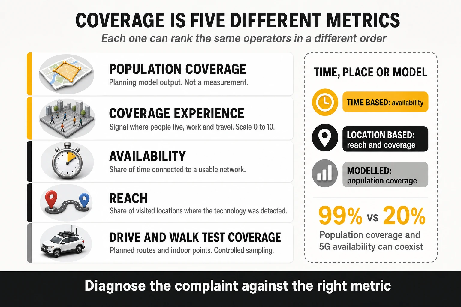
There is a sixth quantity that belongs to the same confusion: the share of tests recorded on a given technology. A low percentage of 5G tests can reflect weak coverage, but it can equally reflect device capability in the panel, subscription eligibility, band configuration, cell-reselection parameters or battery-saving behaviour. Three perspectives have to be kept apart: what has been deployed, what devices actually use, and what quality each technology delivers when it is used. Conflating deployment with usage is the most common error in 5G commentary, in both directions.

Which methodology best represents each dimension

• Peak capacity and physical ceiling: saturation testing. It is the only method designed to find the top of the link.
• Typical everyday speed and availability: passive crowdsourcing, for volume, geographic spread and indoor weighting.
• Mobility — trains, motorways, dense corridors: controlled drive and walk testing, because mobility is sampled by design rather than by accident.
• Stability and consistency: threshold metrics on both sides — Consistent Quality for the installed base, completion-with-quality rates for controlled conditions. Averages from any provider are the wrong instrument.
• Latency under load: saturation testing with explicit loaded-latency phases, complemented by interactivity scoring under application traffic patterns. Sequential suites do not measure it at all.
• Native voice: controlled testing with POLQA scoring, exclusively. No crowdsourced methodology places a native call.
• Video experience: passive panels for scale and model consistency across markets; controlled testing for physical detail — real stalls, real time at 4K, real startup delay on a known device.
• Gaming: controlled measurement toward real game servers for diagnosis; crowdsourced composites for market-level comparison.
• 5G adoption and standalone performance: passive panels for time on 5G and reach at scale; controlled probes for core latency and VoNR behaviour.
• Full digital-experience cycle in one shot: the sequential full test, the only architecture that measures speed, browsing and video as a single user journey.

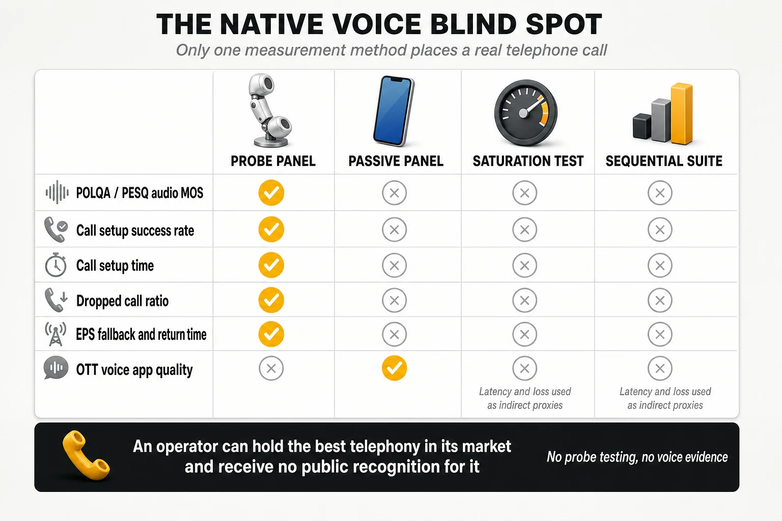
Why the same operator ranks first in one benchmark and third in another

Rank divergence is produced by identifiable mechanisms, each of which can be tested against an operator’s own data:

• Spectrum depth versus spectrum reach. Contiguous mid-band capacity wins saturation tests; strong low-band and dense small cells win availability, consistency and indoor metrics. Different assets, different rankings, same network.
• Server proximity and peering topology. Saturation tests often terminate inside the operator’s network or one hop away; background tests terminate in public clouds and CDNs. Excellent internal transport with poor interconnect leads the first and trails the second.
• Device mix. A base skewed toward older mid-range devices depresses every crowdsourced metric and has no effect on a normalised controlled campaign.
• Indoor weighting. Crowdsourced data is predominantly indoor; drive testing is predominantly outdoor. Operators strong on macro corridors and weak in buildings invert between the two.
• Geographic weighting. One example weight set gives roads 40% of the national result; another gives them 12.5%. That alone can reverse a ranking.
• Threshold versus average. Threshold metrics reward the elimination of bad sessions; averages reward peak performance. An operator that removed its worst 5% of samples moves on the first and barely moves on the second.
• Mapping functions and saturation points. A logarithmic curve compresses a 2x speed advantage into a few points; a linear curve does not.
• Aggregation and tie rules. One-device-one-vote, grid-cell averaging, percentile weighting, minimum-share eligibility and joint-winner conventions each change the answer even when the underlying measurements are identical.

What can be compared directly and what cannot

• Comparable: the direction and magnitude of change over time within a single methodology and an unchanged model; the relative ordering of operators within one market, one methodology and one period; packet loss and jitter when the transport protocol and packet cadence match; and threshold pass rates when the thresholds are identical.
• Not comparable: absolute throughput across methodologies; latency without confirming idle, loaded, one-way or minimum definitions; composite scores with different scales and weightings; coverage metrics with different spatial or temporal bases; award scores across cycles of the same programme; and global rank positions across metrics with different dispersion.
• Comparable only with care: video scores, which rest on different models; and any metric whose provider has revised thresholds, service mix or weights between editions.

Methodology comparison matrix

Attribute	MedUX	Opensignal	Ookla / Speedtest Intelligence	nPerf
Primary architecture	Multi-source: controlled probes, drive and walk tests, fixed probes, SDK crowdsourcing	Passive and active crowdsourcing via SDK in consumer apps	User-initiated saturation plus background telemetry	User-initiated sequential full test
Who triggers the measurement	Scripted scheduler and SDK activation conditions	Nobody: automatic and invisible	The user	The user
Device normalisation	Equivalent models, firmware and tariffs in the controlled leg	None: reflects the installed base	None	4G-capable devices only
Environment weighting	Planned areas, routes and indoor points	Follows user behaviour, indoor-heavy	Wherever the user tests	Wherever the user tests
Latency definition	ICMP RTT and one-way UDP/TWAMP, plus responsiveness under load	One-way UDP and ICMP, hourly cadence	Idle plus download- and upload-loaded RTT	Minimum observed RTT
Consistency metric	Completion and completion-with-quality against qualifier thresholds	Consistent Quality, Core and Excellent threshold sets	Consistency Score against minimum thresholds	Browsing and streaming success percentages
Composite construction	Qualifier and differentiator KPIs to service scores to weighted global score, with source visibility	Metric-level reporting; no single global composite	Speed Score from percentiles, download 70% / upload 20% / latency 10%	Logarithmic points composite across the three phases
Native voice	Real calls with POLQA scoring and full ETSI voice KPI set	Not measured; OTT voice only	Not measured	Not measured
Statistical treatment	Confidence and margin calculated and disclosed per deployment	Joint winners when differences are not significant; no reporting when intervals are large	Minimum sample share and geographic spread for eligibility	Declared precision per barometer
Technology discrimination	Modem-level RRC and core attachment state	Time on 5G and 5G SA from device telemetry	Primary and secondary cell detection via OS APIs	OS 5G indicator
Best used for	Engineering audit, SLA verification, native voice, converged fixed and mobile	Installed-base experience, coverage, availability, consistency	Capacity ceiling, bufferbloat, market-level speed	End-to-end digital experience per test cycle
Main blind spot	Sample volume and route dependency in the controlled leg; source weighting in the combined score	Does not measure the physical ceiling; no native voice	Self-selection; no application QoE beyond composites	No loaded latency, no voice, urban skew

12. Application-level benchmarking, including AI services

Seven questions every service test has to answer

Service-level testing is where methodologies differ most and document least. A homogeneous template makes any test case auditable:

1. What exact operation is executed?
2. Against which target, hosted where, reached over which path?
3. When does the clock start and when does it stop?
4. What counts as success?
5. What counts as acceptable quality — the qualifier?
6. Which KPIs separate good from excellent — the differentiators?
7. Which factors outside the network can change the result?

Question three is the one most often skipped and the most consequential. A call setup time measured from the user interface and one measured at the signalling layer differ by the processing time of the device software; a page load measured to “fully rendered” and one measured to “first megabyte downloaded” are different experiments on the same page. Published frameworks address this explicitly, defining browsing success as downloading at least 1 MB of page content within a time limit rather than as a complete page load, precisely because modern pages never finish loading in a comparable way.

Service	Minimum success	Differentiators	Methodological caution
File download and upload	Transfer completed and minimum throughput achieved	P10 and P90 of throughput, share of samples above speed tiers, session duration	Number of parallel flows and distance to the server change the result more than the radio does
Web browsing	Page content accessed and a defined volume downloaded within the time limit	DNS time, TTFB, time to first megabyte, full load time	Page set composition, JavaScript weight, third-party resources and CDN hosting
Video streaming	Playback started, no freeze above the duration threshold	Access time, average resolution, time at maximum resolution, freezing proportion	Adaptive bitrate logic, device capability and content availability also decide resolution
Gaming and interactivity	Interactivity score above the floor under an application traffic pattern	Average interactivity score, latency variation, loss and the unfavourable latency tail	Server location and traffic pattern selection determine the absolute values
Native voice	Composite: setup success, setup time under threshold, not dropped, no consecutive very low speech samples	P10 of MOS, P90 of setup time, drop ratio, fallback behaviour	Codec negotiation, IMS configuration and mobility events dominate the result
Social media and messaging	Activity completed within the duration threshold	Average duration, share of activities above a long-duration threshold	Platform-side processing time is included in the measurement and is identical for all operators
Generative AI services	Response obtained without error inside the timeout	Time to first token, delivery regularity, total response time	Model, prompt length, output length, service load and inference location all move the result

Two video cautions worth stating explicitly

• A stall-free session does not mean good visual quality. A player that settles at 480p and never interrupts will score perfectly on freezing metrics and badly on resolution metrics. This is why scoring frameworks combine a success criterion based on freezes with a separate resolution indicator — in one published example set, average video resolution carries 27% of the video score, against 55% for the composite success criterion.
• A low share of time at maximum resolution does not prove the network caused it. Adaptive bitrate algorithms are conservative by design, device decoding capability sets a ceiling, and not every title is available in every resolution. Attributing resolution shortfalls to the radio network without eliminating those three explanations is a diagnostic error that leads to wasted capacity investment.

Interactivity scoring: the standardised way to measure gaming

Gaming measurement has moved beyond “ping to a game server”. ITU-T G.1051 specifies continuous measurement of two-way latency, latency variation and loss over a defined observation period — using a UDP stream reflected by a far-end server, with TWAMP as one possible basis — and feeds the results into a model that expresses interactivity as a single figure of merit. Critically, the model is not generic: it is scaled per use case, and the measurement result depends on the traffic pattern chosen to emulate the application, so the Recommendation also defines rules for deriving those patterns.

Published example weight sets already treat this as a first-class service category. One set includes an interactivity “eGaming pattern” worth 5% of data services, scored as the percentage of tests achieving an interactivity score above zero — with a bad limit of 60% and a good limit of 95% — plus the average interactivity score across all samples, mapped between 25 and 75. Two consequences follow for operators: gaming performance is now measurable in a standardised way rather than by proxy, and absolute scores are only comparable between campaigns using the same traffic pattern.

OTT conversational applications as a separate category

Voice over messaging applications is now scored as its own service, separate from native telephony. One published example set assigns it 5% of data services and scores it with a composite call success criterion — setup success, setup time under 15 seconds, the inverse of the drop ratio, and the ratio of calls with no two consecutive speech samples below 1.3 MOS — at 55%, plus the 10th percentile of MOS across all samples, mapped between 2.0 and 4.0 MOS, at 45%. Speech quality for these services can be estimated with the machine-learning model defined in ITU-T P.565.1 rather than by injecting reference audio.

The structural point is that an operator now has two voice scores with different mechanics and different owners. Native voice depends on IMS, codecs, QoS enforcement and mobility; OTT voice depends on latency, loss, jitter and the path to the application platform. They can diverge sharply in both directions, and a strategy that optimises one does not automatically improve the other.

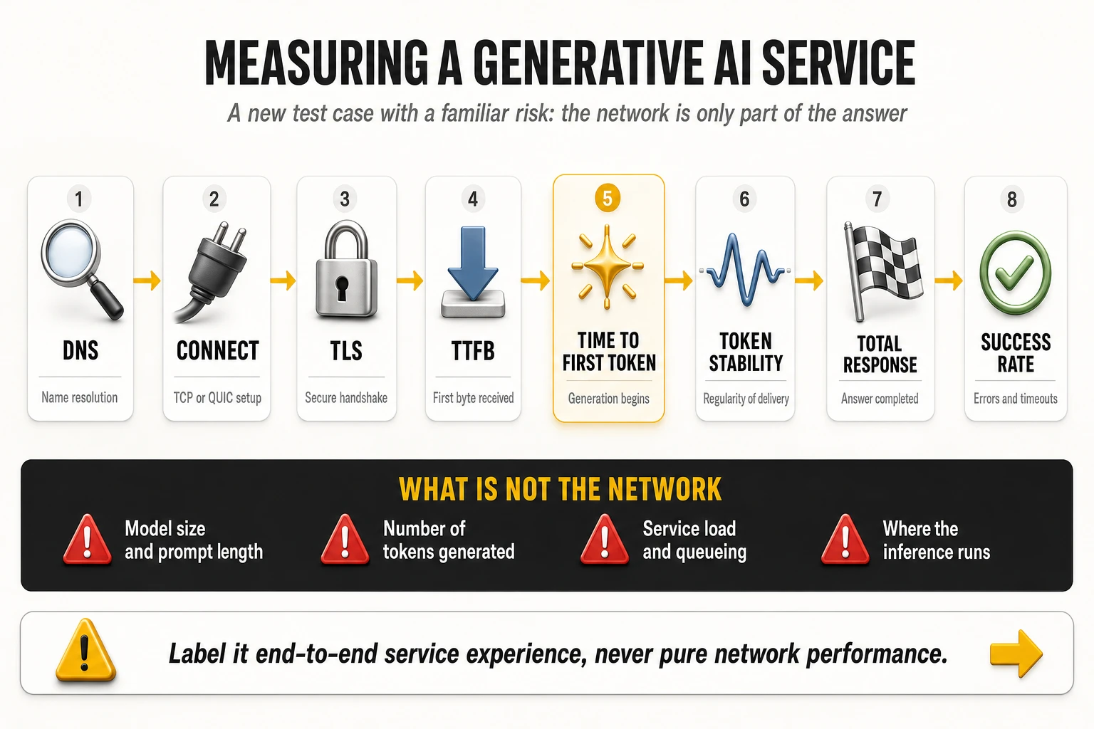
Generative AI: a new service category with a familiar trap

Conversational AI assistants have become a daily digital activity, and benchmarking is beginning to treat them as a test case in their own right — one benchmarking provider has publicly stated that future editions of its framework will add assessment areas including AI readiness. The measurement chain decomposes cleanly:

• DNS resolution time: resolving the service endpoint.
• Connection establishment and TLS handshake time: transport and security setup, increasingly over QUIC rather than TCP.
• Time to first byte: the first response from the platform.
• Time to first token: when the answer actually starts appearing — the moment the user perceives as “it responded”.
• Token delivery stability: the regularity of the stream. An answer delivered in smooth increments feels faster than one delivered in bursts with the same total duration.
• Total response time, completion success and timeout or error rate: the end-to-end outcome.

The trap is attribution, and it is more severe here than in any other service. Response time for an AI assistant depends on the model being served, the length of the prompt, the number of tokens generated, the load on the service at that moment, the location where inference runs, possible reuse of cached responses, and routing to different back-end clusters. None of those are network variables. A benchmark that measures total response time across operators without controlling or at least observing them may be measuring differences between inference clusters and reporting them as differences between networks.

Three rules make the category usable rather than misleading:

• Fix the prompt and the model. Identical prompts, identical requested output length, identical service tier, executed simultaneously on the operators compared — the same discipline a controlled campaign already applies to video assets and file sizes.
• Report the network-attributable phases separately. DNS, connection, TLS and time to first byte are dominated by the network and the path; time to first token and total response time are not. Publishing them separately is what turns an ambiguous number into a diagnosis.
• Label the metric honestly. It is end-to-end experience of a specific service, not network performance. That label is not a weakness — it is the same status that browsing and social media metrics have always had, where the measurement inevitably includes platform processing time that is identical for all operators under test.

For operators there is a strategic reading underneath the methodological one. If AI assistants become a scored service category in public benchmarks, the levers that move the score are DNS proximity, peering with the AI platforms, edge breakout and uplink performance for prompt and context upload — the same interconnect-side investments that already decide browsing and video scores, applied to a new destination set. The operators that treat AI endpoints as a peering and caching problem will see it in their scores before their competitors understand why.

13. Engineering actions that improve each metric

The section below pairs every benchmark dimension with the engineering levers that move it and with the internal counters that prove whether the action worked. The verification discipline matters as much as the action: a change that improves a benchmark score three months later, with no internal counter moving in between, is indistinguishable from luck.

Downlink throughput

• Channel bandwidth first. Contiguous mid-band spectrum is the dominant term in cell capacity. Deploying 80–100 MHz in the 3.5 GHz C-band (3GPP band n78) is the single highest-impact action on peak and median download speed, because throughput scales close to linearly with bandwidth at a given spectral efficiency.
• Massive MIMO where traffic density justifies it. Replacing passive panels with 32T32R or 64T64R active antenna systems in dense urban sites multiplies cell capacity through 3D beamforming and multi-user spatial multiplexing. Beamforming concentrates energy on the user, with SINR gains above 12 dB reported in favourable conditions (industry estimates); MU-MIMO then serves up to sixteen spatially multiplexed layers in the same cell, which is what actually raises busy-hour throughput rather than peak throughput.
• Carrier aggregation across bands. Three- and four-component NR carrier aggregation — for example n78 plus a second mid-band carrier plus a low-band anchor — multiplies the effective bandwidth available to a capable handset; three- and four-carrier aggregation is what produces peaks above 1.5 Gbps in saturation tests on compatible devices (industry estimates).
• High-order modulation with the radio conditions to support it. 256-QAM in downlink adds roughly a third more bits per symbol than 64-QAM, but only where SINR is high enough to sustain it — clean conditions above about 22 dB. Enabling high-order modulation on a network with dirty interference conditions produces retransmissions, not throughput.
• Transport dimensioning behind the radio. A 64T64R site on a congested 1 Gbps backhaul link is a capacity problem disguised as a radio investment. Fronthaul and backhaul must be dimensioned for the aggregate busy-hour cell throughput, not for the average.

Verify with: cell and user average spectral efficiency (bit/s/Hz), PRB utilisation at busy hour, CQI and MIMO rank distribution, the percentage of samples above the benchmark’s excellence thresholds, and the P10 of the download distribution — which is the number that moves benchmark consistency scores, unlike the average.

Uplink throughput: the metric most benchmarks now punish

Uplink has become the discriminating dimension, because video calling, social publishing, cloud sync and machine-generated traffic all push upstream, while TDD frame configurations and legacy access plant were engineered downstream-heavy. The levers:

• Two-layer uplink MIMO on 5G Standalone. Enabling a 2Tx profile on the handset over dedicated NR carriers delivers up to 2.2 times the uplink capacity of the single-layer uplink typical of non-standalone deployments, where the uplink is frequently anchored on the LTE carrier, and supports uplink rates above 120 Mbps in favourable radio conditions (industry estimates).
• Uplink carrier aggregation and supplementary uplink. Combining a low-band FDD carrier for uplink reach with a mid-band TDD carrier for uplink capacity extends usable uplink to cell edge, where the mid-band uplink budget collapses first.
• TDD frame pattern review. Slot patterns that allocate around three quarters of slots to downlink cap uplink regardless of any other optimisation. Re-balancing requires cross-operator coordination to avoid interference, which is exactly why it is rarely done and why it remains a differentiator for those who do it.
• Uplink-specific radio features: higher-order uplink modulation where SINR allows, power-control tuning, and uplink coverage enhancement on low band to protect the cell-edge distribution.

Verify with: uplink PRB utilisation, uplink SINR and power-headroom distributions, the share of sessions above the benchmark upload threshold (1.5 Mbps is the common excellence floor), and uplink P10 at cell edge.

Idle latency

• Move the user plane closer to the radio. Distributing the User Plane Function of the 5G core to regional or edge sites removes long-haul transit from every packet and typically takes 8 to 15 ms out of baseline round-trip time (industry estimates).
• Migrate to 5G Standalone. Non-standalone attachment keeps session management and control signalling on the 4G core, with control-plane latency commonly in the 15 to 35 ms range because of dual connectivity; a native 5G core with direct NR connectivity brings it to roughly 5 to 12 ms (industry estimates).
• Shorten the path to content. Direct peering at internet exchange points with the major content, cloud and gaming platforms removes transit hops. Each avoided hop is both latency and a potential congestion point.
• Radio-side scheduling. Shorter transmission time intervals, pre-scheduling and grant-free uplink access reduce the access delay component that dominates on lightly loaded cells.

Verify with: per-segment latency decomposition (radio, transport, core, interconnect) rather than end-to-end RTT alone, traceroute hop counts toward the top traffic destinations, and the latency distribution below the 50 ms threshold used by consistency metrics.

Latency under load: eliminating bufferbloat

Bufferbloat is the gap between idle and loaded latency, and it is the most under-managed quality problem in mobile networks. When buffers in the radio scheduler, the aggregation router or the CPE fill under load, queuing delay can push round-trip time from tens of milliseconds to several hundred, destroying video calling, cloud gaming and any interactive session that shares the link with a download. The fixes are well standardised and rarely deployed end to end:

• Active queue management. Deploying CoDel or FQ-CoDel in transport aggregation routers and in the base station MAC layer drops or marks packets before queues saturate. Reported effects take latency under load from above 300 ms to under 40 ms on the same link (industry estimates), holding delay to a small multiple of idle latency instead of an order of magnitude above it.
• L4S. The Low Latency, Low Loss, Scalable throughput architecture uses explicit congestion notification to signal congestion to the sender before queues build, keeping latency under load below roughly 15 ms even during heavy transfers (industry estimates). It requires coordinated support in the RAN, the core user plane and the content endpoints, which is why it separates the operators that treat responsiveness as a product feature from those that treat it as a side effect.
• Buffer sizing and scheduler tuning in the radio, so that per-user queues are dimensioned for the actual bandwidth-delay product rather than for the worst-case legacy assumption.

Verify with: the ratio of loaded to idle latency in the download and upload phases, the 95th percentile of queuing delay per aggregation node, and the gaming and video-calling scores that depend on it.

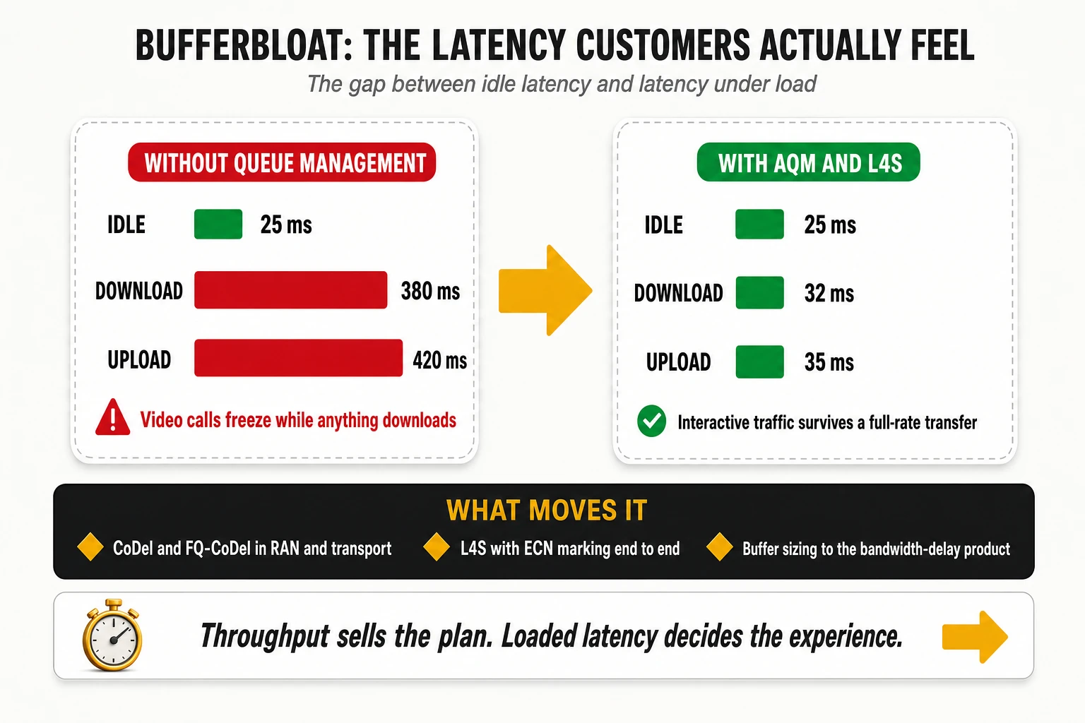
Jitter and packet loss

• Interference control in the radio. Most jitter and loss on a healthy transport network originates in the air interface: overlapping coverage, PCI collisions and confusion, uplink interference from misconfigured power control, and external interference sources. Systematic PCI and neighbour-relation audits, remote electrical tilt optimisation and interference hunting move these KPIs more than any transport action.
• Retransmission and duplication mechanisms. PDCP duplication on critical bearers and robust header compression on voice bearers reduce effective loss for the traffic that cannot tolerate it.
• Transport quality. Consistent QoS marking end to end, protected rings or fast-reroute in the aggregation layer, and microwave link budget review where fibre is not available — degraded microwave hops are a classic source of intermittent loss that looks like a radio fault.
• Peering quality. Loss introduced at congested transit interconnects is invisible in RAN counters and fully visible in benchmark results, because crowdsourced tests terminate beyond the operator’s border.

Verify with: UDP-based one-way loss and consecutive-pair jitter per region, radio block error rate and HARQ retransmission rates, interference-over-thermal levels per cell, and interconnect utilisation at the 95th percentile.

Consistency, stability and reliability

Threshold metrics respond to a completely different engineering programme from average metrics, and this is where most operators misallocate effort. Consistency improves when the worst sessions disappear, not when the best sessions improve. The programme that moves it:

• Work the failure tail, not the average. Identify the cells, hours and locations producing samples below 5 Mbps download, above 50 ms latency, above 12 ms jitter or above 1% discard, and treat those as a defect backlog with owners and deadlines. A small number of cells usually produces a disproportionate share of failing samples.
• Attack session failures separately from slow sessions. Consistency metrics multiply the pass rate by the completion rate, so a session that never completed costs more than a slow one. Setup failures, radio link failures and DNS timeouts belong in a different queue from congestion.
• Guarantee the floor at busy hour. Load balancing across carriers and layers, admission control that protects the minimum rather than maximising the peak, and capacity triggers based on the percentage of users below threshold rather than on average cell load.
• Protect time-to-first-byte. TTFB is part of the excellence threshold set, and it is determined by DNS, TLS handshake and content proximity rather than by the radio.

Verify with: percentage of samples passing all thresholds simultaneously, test completion ratio, the count of cells contributing more than a defined share of failing samples, and the trend of the 10th percentile across every core KPI.

Coverage, availability, reach and indoor performance

• Low-band refarming for 5G. Deploying 5G on 700 MHz or another low band with 10–15 MHz of bandwidth transforms reach and availability metrics, because propagation and in-building penetration — not capacity — are what those metrics measure. Mid-band alone produces excellent speed scores and mediocre availability scores.
• Selective, not universal, dynamic spectrum sharing. DSS lets 4G and 5G share one carrier and is the fastest route to a 5G icon on the handset, but the signalling overhead it introduces — commonly estimated at 15% to 20% of capacity — makes it a poor choice in congested areas. Dedicated clean carriers outperform it wherever spectrum allows.
• Indoor systems where the traffic is. Small cells and distributed antenna systems in shopping centres, transport hubs, stadiums and corporate buildings address the environment that generates around 80% of mobile traffic (industry estimates) and where crowdsourced availability metrics do most of their sampling.
• Coverage-hole closure through automation. Self-organising network algorithms for remote electrical tilt and power management close gaps continuously rather than through annual planning cycles, and minimisation-of-drive-test reporting from handsets (3GPP TS 37.320) provides the geolocated evidence without sending a vehicle.
• Idle-mode and re-selection parameters. Availability is a time-based metric, so camping behaviour matters as much as footprint: priority settings that park devices on a layer with poor indoor penetration will depress availability even where coverage exists.

Verify with: percentage of time on 4G/5G per device class, no-signal rate, 5G availability and 5G reach trends, geolocated RSRP/SINR distributions from handset reporting, and in-building sample counts before and after deployment.

Congestion management at busy hour

• Predictive rather than reactive capacity triggers: forecasting cell-level congestion weeks ahead from traffic growth, PRB utilisation trends and event calendars, so capacity lands before the degradation rather than after the complaint.
• Layer and carrier load balancing tuned on user-experience thresholds instead of on cell load, so users are moved when their session quality is about to fail, not when a counter crosses an arbitrary percentage.
• Traffic offload: on-net caching and carrier Wi-Fi where relevant, removing volume from the busy-hour radio budget entirely.

Verify with: the ratio between busy-hour and idle-hour results for every key metric — which is precisely the split some benchmarks publish by default, making it an externally auditable KPI rather than an internal one.

Web browsing, DNS and time-to-first-byte

Browsing scores are won and lost outside the radio network, which is why they are frequently the cheapest benchmark points available to an operator. A page load is a sequence of DNS resolutions, TCP or QUIC handshakes, TLS negotiations and dozens of object fetches; the radio contributes bandwidth, and almost everything else contributes delay.

• Anycast recursive DNS inside the mobile network, with aggressive local caching and prefetching. DNS resolution can represent up to 40% of total page load time on mobile (industry estimates), and moving resolution from a distant resolver to an on-net anycast farm brings it below 5 ms.
• On-net CDN caches and direct peering. Hosting content caches at aggregation sites and peering directly with the largest content and cloud platforms is the main lever on time-to-first-byte, which is a threshold component of consistency metrics as well as a browsing determinant. Edge caches bring TTFB into the tens of milliseconds and video start time below one second (industry estimates), against thresholds of 800 ms for TTFB in the excellence threshold sets.
• Modern congestion control on operator-side servers and proxies. Replacing loss-based congestion control with BBR-class algorithms improves throughput on lossy mobile paths without inflating queues, which improves page load and avoids making bufferbloat worse.
• QUIC-aware transport handling, since a growing share of web and video traffic runs over UDP-based QUIC and is invisible to middleboxes tuned for TCP.

Verify with: DNS resolution time distribution, TTFB percentiles by destination, page load time for the site set used by the benchmark, and cache hit ratio on on-net CDN nodes.

Video experience

Video scores decompose into three measurable components — start time, resolution sustained and stall behaviour — and each has a distinct cause.

• Start time is dominated by DNS, TTFB and the time needed to fill the initial buffer. On-net caching addresses all three at once; it is the highest-leverage action on video scores.
• Resolution sustained is a function of the steady-state throughput the adaptive bitrate algorithm observes, and of its stability. A link that oscillates between 30 and 3 Mbps will settle at a lower resolution than a link that holds 8 Mbps steadily — which is why consistency work improves video scores more than peak capacity work.
• Stalls come from throughput collapses and from packet loss during buffer refill, typically at handover, at cell edge or during congestion spikes. Mobility robustness and interference cleanup are the relevant levers, not capacity.
• Traffic management transparency. Any policy that shapes or transcodes video will show up directly in video scores and in the time-at-maximum-resolution KPI, and benchmark panels will detect it regardless of how it is described commercially.

Verify with: video start time percentiles, percentage of session time at full resolution, stalls per hour and mean time between stalls, and stall correlation with handover events.

Gaming

• Direct interconnection with the game platforms. Gaming scores measure the path to specific production servers. Direct peering with the major publishers and cloud gaming providers at the nearest exchange point removes transit hops and the jitter that transit congestion introduces.
• Edge user plane and local breakout, so that gaming traffic does not traverse a national core before exiting to a regional game server.
• Jitter discipline over raw latency. Players tolerate a stable 40 ms far better than a fluctuating 25 ms. Queue management and scheduler consistency matter more than absolute distance once latency is below roughly 50 ms.
• Differentiated QoS for interactive traffic, using 5G QoS identifiers designed for low-latency interactive services, and network slicing where the commercial model justifies it.

Verify with: median and 90th or 95th percentile latency to named game endpoints — the unfavourable tail, not the best tenth, jitter and loss on those same paths, and hop count changes after peering adjustments.

Native voice: VoLTE and VoNR

Voice is the dimension where an operator can differentiate most and is measured least, which makes it both an opportunity and a risk. Only probe-based audits will detect the improvement — but customers detect it immediately, because a failed or delayed call generates a call to customer care in a way that a slow download does not.

• Deploy wideband and super-wideband codecs. Enabling EVS (Enhanced Voice Services) in super-wideband or full-band mode across the IMS core and in device SDP negotiation raises perceived audio quality substantially above traditional narrowband and AMR-WB coding — the difference between a call that sounds like a telephone and one that sounds like the person is in the room. Reported effects move POLQA MOS from around 3.8 to above 4.3 on the same network (industry estimates), which on a 1-to-5 scale is the largest single-action improvement available in any quality programme.
• Enforce QoS end to end for voice bearers. Strict QCI 1 / 5QI 1 treatment for the media bearer and QCI 5 / 5QI 5 for SIP signalling, honoured on the radio interface and preserved in IP transport marking, protects voice from data congestion in the same cell.
• Tune IMS signalling. SIP timer optimisation, registration handling and radio bearer assignment sequencing reduce call setup time. Setup times in the 1.2 to 1.5 second range are an achievable engineering target and are measurable from the first day of the change.
• Move from EPS fallback to native VoNR on 5G Standalone. Fallback forces a 5G-attached device to move to LTE before the call connects, adding delay to setup and interrupting the data session. Native voice over New Radio removes both effects, cutting roughly 1.5 seconds from the setup delay (industry estimates), and is one of the few 5G features whose benefit a customer perceives without being told.
• Optimise mobility for voice specifically. Most drops are handover events. Neighbour lists, A3/A5 event thresholds, time-to-trigger and inter-RAT fallback parameters need a voice-specific review rather than the data-oriented default.

Verify with: POLQA MOS distribution and the share of calls below the acceptability floor, call setup success rate, call setup time percentiles, drop call rate by cause code, EPS fallback rate and fallback duration, and codec negotiation statistics showing what share of calls actually establish on the wideband codec.

5G Standalone experience

Standalone architecture is the enabler behind several benchmark dimensions at once, which is why it deserves its own programme rather than being treated as a core upgrade. Non-standalone keeps the control plane on the 4G core with dual connectivity, which limits latency, restricts uplink and raises device power consumption during tests. Standalone removes those constraints and unlocks network slicing, edge user-plane placement and native voice.

• Migrate traffic, not just capability. Deploying a 5G core is not the same as having users on it. The metric that matters is time on 5G SA, and it is driven by device support, subscription provisioning and — critically — by re-selection and handover parameters that keep capable devices attached to the standalone layer.
• Tune retention thresholds. RSRP thresholds for A3/A5 events determine whether devices stay on 5G or drop to 4G at the first weak sample, and they are the difference between a high and a low 5G availability figure on the same physical network.
• Pair standalone with low-band coverage. Standalone on mid-band alone produces excellent speed and poor availability; the combination of low-band standalone coverage and mid-band standalone capacity is what moves both families of metric.

Verify with: percentage of time on 5G SA versus NSA for capable devices, SA versus NSA latency and uplink comparisons on the same sites, VoNR penetration, and slice-level KPIs where slicing is commercially deployed.

Mobility, handovers and parameterisation

• Mobility robustness optimisation: automated detection and correction of too-early, too-late and wrong-cell handovers, which are the root cause of most drops, stalls and throughput collapses observed in mobility scenarios.
• Automatic neighbour relations maintained continuously, since missing neighbours produce drops that look like coverage holes and are cured with a database entry rather than a site.
• Corridor-specific parameter sets for motorways and rail lines, where Doppler, cell dwell time and handover frequency differ so much from static urban use that a single parameter set cannot serve both.
• Random access and re-establishment tuning, which determines how quickly a session recovers after a radio link failure rather than whether it fails at all.

Verify with: handover success rate by type and by neighbour pair, radio link failure rate, re-establishment success rate, and throughput and stall behaviour measured specifically on mobility routes rather than network-wide.

SON, closed-loop automation and applied AI

Manual optimisation cannot hold a quality target across tens of thousands of cells with daily traffic variation; the question is not whether to automate but which loops to close first.

• Closed-loop SON for the repetitive cases: tilt and power optimisation, load balancing, neighbour management, PCI conflict resolution and energy-saving state changes. These are well-understood control problems with measurable objectives and should run without human approval once trusted.
• RAN intelligent controller architectures that let optimisation applications act on near-real-time radio state, rather than on counters aggregated at fifteen-minute granularity.
• Machine learning where the pattern is statistical, not deterministic: congestion forecasting, anomaly detection across counter sets too large for human inspection, cell-level degradation prediction, and root-cause classification that correlates radio, transport and core symptoms into a single incident.
• Predictive maintenance on the physical plant: power supplies, batteries, cooling and antenna line systems, where failure signatures appear in telemetry days before service degrades.
• Proactive customer action: detecting degradation at the level of individual subscribers or sites and acting before complaints arrive, which converts a quality programme into a churn programme.

Verify with: percentage of optimisation actions executed without human intervention, mean time to detect and mean time to repair, share of incidents detected before the first customer complaint, and the proportion of capacity upgrades triggered by forecast rather than by alarm.

End-to-end observability: the precondition for everything above

None of these actions can be prioritised without a data layer that connects radio counters, transport telemetry, core signalling traces, application-layer measurement and external benchmark feeds into one addressable model. The practical requirements are unglamorous and decisive: geolocated per-session records rather than cell aggregates; correlation keys that survive across RAN, transport, core and IMS domains; retention long enough to compare against a quarterly benchmark cycle; and a single definition of each KPI shared by engineering, marketing and customer operations. An operator that cannot reproduce its own benchmark result from internal data cannot manage it — it can only react to it.

Action-to-metric map

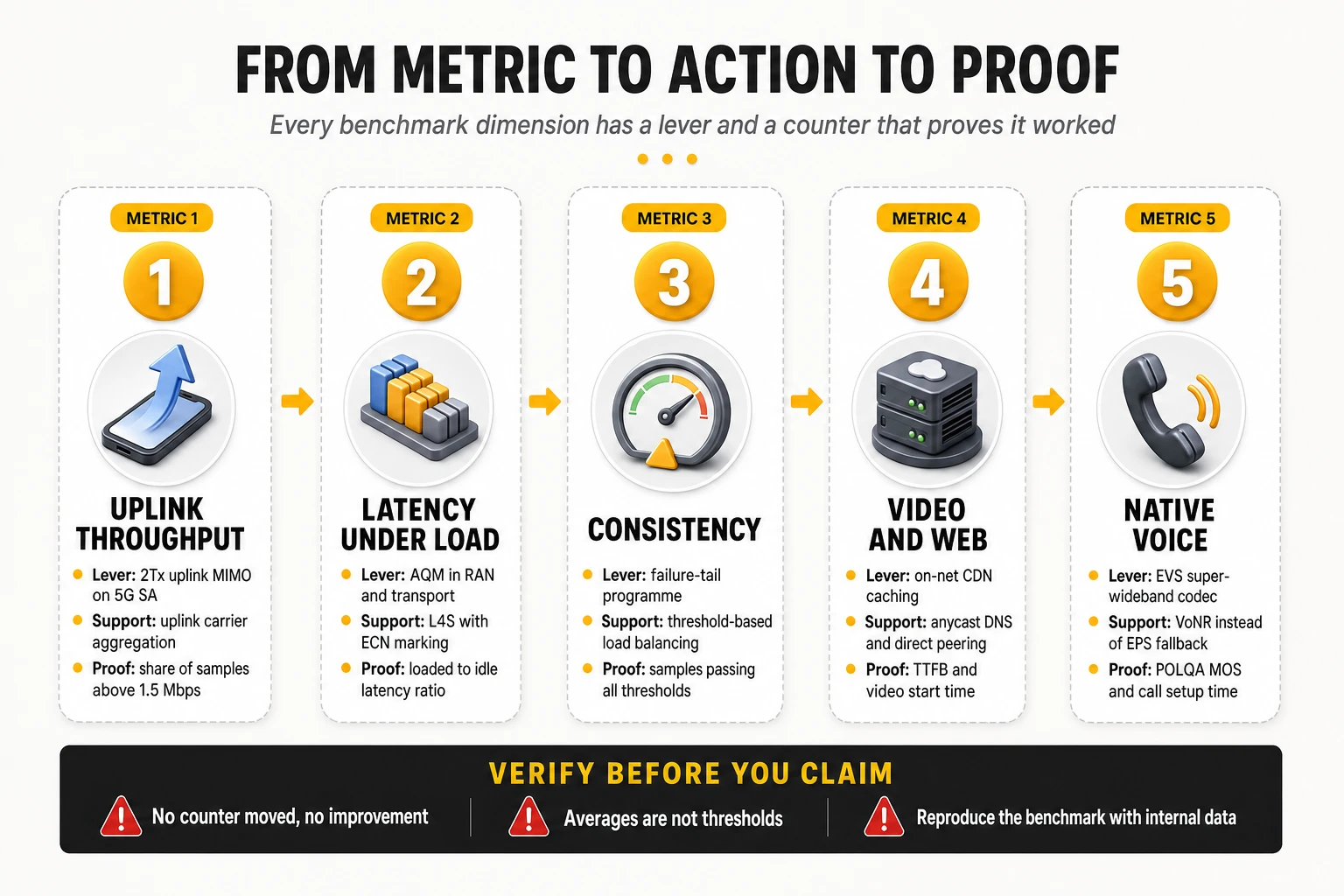
Target metric	Primary engineering lever	Secondary lever	Verification KPI
Download throughput	80–100 MHz mid-band plus 64T64R massive MIMO	3–4 carrier NR aggregation, 256-QAM	Spectral efficiency, PRB utilisation, rank distribution, DL P10
Upload throughput	2Tx uplink MIMO on 5G SA	Uplink CA with low band, TDD pattern review	UL SINR, power headroom, % samples above 1.5 Mbps
Idle latency	Edge user plane / distributed UPF	5G SA migration, direct IXP peering	Per-segment latency decomposition, hop count
Latency under load	AQM (CoDel / FQ-CoDel) in RAN and transport	L4S with ECN marking, buffer resizing	Loaded-to-idle latency ratio, queuing delay P95
Jitter and packet loss	Interference and PCI cleanup, tilt optimisation	Transport QoS, peering capacity, PDCP duplication	One-way loss, consecutive-pair jitter, BLER, HARQ retransmissions
Consistency / reliability	Failure-tail elimination programme on worst cells and hours	Threshold-based load balancing and admission control	% samples passing all thresholds, completion ratio, KPI P10
Availability and reach	Low-band 5G refarming	Indoor small cells and DAS, idle-mode parameters	Time on 4G/5G, no-signal rate, 5G availability and reach
Coverage experience	Densification where users actually are	SON tilt and power automation, MDT-based hole detection	Geolocated RSRP/SINR distribution, indoor sample quality
Web and TTFB	On-net CDN caching and direct peering	Anycast DNS, BBR-class congestion control	DNS time, TTFB percentiles, cache hit ratio
Video experience	Edge caching to cut start time	Throughput stability and handover robustness	Start time, % time at full resolution, stalls per hour
Gaming	Direct peering with game platforms	Edge breakout, interactive QoS, jitter control	P50 and P90 latency to game endpoints, jitter, loss
Native voice	EVS super-wideband codec end to end	5QI 1 enforcement, SIP timer tuning, VoNR over EPS fallback	POLQA MOS, CSSR, setup time, drop rate, fallback rate
5G experience	Traffic migration to standalone core	Retention thresholds, low-band SA coverage	Time on 5G SA, SA vs NSA latency and uplink deltas
Mobility performance	Mobility robustness optimisation and ANR	Corridor-specific parameter sets	Handover success by pair, radio link failure rate
All of the above, sustainably	Closed-loop automation with defined objectives	ML forecasting and anomaly detection, predictive maintenance	Autonomous action share, MTTD/MTTR, pre-complaint detection rate

14. Benchmark leaders: who leads each dimension, and why

Two reading rules apply to everything in this section. First, every figure belongs to a specific award cycle and a specific methodology; scores move between cycles because panels, device mixes and models change, so a value should never be compared across cycles or across providers. Second, leadership in one dimension says nothing about the others — the operators that dominate speed tables are frequently not the ones that dominate reliability or consistency tables, and that divergence is the most useful information in the whole exercise.

Second, award tables are structured, and the structure explains most of what looks surprising in them. The largest crowdsourced programme splits operators between markets above and below 200,000 km² of land area, names a Winner per category and division, a Leader tier below it and Rising Stars for the biggest year-on-year improvements, and declares joint winners wherever a difference is not statistically significant. A “shared first place” among a dozen operators is not a quirk of the data; it is the tie rule working as designed.

The most recent award cycle, read structurally

The 2026 5G awards, built on measurements collected between 1 January and 29 June 2026, illustrate every point made in the methodological sections above:

• 5G Download Speed: SK Telecom (South Korea) in the small land-area division, with a reported 495.1 Mbps; Vivo (Brazil) in the large land-area division. Two different engineering stories — extreme site density on one side, wide contiguous mid-band concentrated in metropolitan areas on the other — and they are not in competition with each other because the division rule separates them.
• 5G Coverage Experience: T-Mobile (United States) among large land-area markets and Singtel (Singapore) among small ones — the clearest possible demonstration of why land area is treated as a structural variable rather than as part of the score.
• Time on 5G, new in the 2026 edition: T-Mobile (United States) and StarHub (Singapore). This is the metric that separates deployment from usage, and its arrival as an award category is an acknowledgment that 5G speed alone had stopped being informative.
• 5G Reliability: au and SoftBank (Japan) jointly in the large division; Telenor and Norlys (Denmark), A1 (Austria) and A1 (Slovenia) jointly in the small division. Four of those six are mid-sized European operators, which is the strongest available evidence that reliability leadership is not a function of scale or spectrum wealth.
• 5G Video Experience: Odido (Netherlands) alone in the small division, against twelve joint winners across Finland, Poland, Sweden and Norway in the large division. The twelve-way tie is the statistical rule from section 6 made visible: at the top of the video scale, the differences between operators are no longer distinguishable from zero.
• 5G Games Experience: Telekom (Germany) in the large division and Swisscom (Switzerland) in the small one — both markets where interconnect density and short paths to regional game platforms matter more than radio capacity.
• 5G Voice App Experience: au (Japan) and KT (South Korea). Note the category: this is over-the-top voice quality, not native telephony, and it says nothing about VoNR performance.

In the companion all-technology awards covering the second half of 2025, one operator — au (KDDI, Japan) — took the top rating in four of the eight categories: reliability, voice app, games and time on 4G/5G, two of them jointly. The pattern across both cycles is consistent and worth stating as a finding rather than a list: the operators that accumulate awards do so in the reliability, latency and time-on-technology families, not in peak speed. Speed leadership rotates with spectrum auctions and refarming; consistency leadership persists, because it is produced by density, transport design and operating discipline that take years to build and do not evaporate when a competitor lights up a new band.

The figures quoted in the remainder of this section come from earlier award cycles and are retained because they illustrate the mechanisms, not because they describe the current table. Any specific value should be checked against the most recent publication before being used in a competitive analysis.

Download speed

• South Korea — SK Telecom, KT and LG U+. Korean operators have held the top of global download tables for years. Reported values in recent Opensignal global award cycles place the leading Korean operator’s Download Speed Experience around 192 Mbps, a figure driven by the highest density of 5G cells per square kilometre in the world, 64T64R massive MIMO on 3.5 GHz and 10 Gbps fibre fronthaul. Their competitive gap is not spectrum — it is site density.
• United States — T-Mobile. Global winner for 5G Download Speed among large-geography markets in recent cycles, with reported 5G download around 152 Mbps, and repeatedly recognised in Ookla’s Speedtest Awards as the country’s fastest mobile network and best 5G network. The technical basis is a 2.5 GHz mid-band position (band n41) acquired early, nationwide standalone 5G, and three-carrier NR aggregation combining mid-band and low-band carriers.
• Brazil — Vivo. Reported as sole winner for 5G Download Speed among large-geography markets in a recent cycle at roughly 362 Mbps, built on 100 MHz of contiguous 3.5 GHz standalone spectrum concentrated in metropolitan areas with high-power massive MIMO. It is the clearest illustration that contiguous mid-band bandwidth, not average network quality, determines peak speed leadership.
• Gulf markets — United Arab Emirates, Qatar, Kuwait. In Ookla’s Speedtest Global Index, Gulf markets have consistently occupied the top positions for median mobile download speed, ahead of Korea and well ahead of Western Europe. The drivers are wide mid-band holdings, extensive millimetre-wave deployment in dense districts, compact geography and a device base skewed to recent flagships.

Upload speed

• Finland — DNA. Reported as global winner for Upload Speed Experience at roughly 19.4 Mbps in a recent cycle. Nordic operators dominate this metric for a structural reason: heavy uplink usage per subscriber, mid-band layers configured with uplink capacity in mind, and dense fibre backhaul.
• Norway — Telenor. Reported global upload winner in an earlier cycle at approximately 19.3 Mbps, with the same underlying combination of uplink-oriented configuration and modernised transport.
• South Korea — SK Telecom. Reported around 27 Mbps upload in a recent cycle, the highest of the leading markets, attributable to two-layer uplink MIMO on standalone 5G combined with 10 Gbps fibre backhaul.

The gap between global leaders at roughly 19–27 Mbps and typical European upload figures in the single digits is the widest relative gap in the entire benchmark landscape, and it is the dimension where a European operator can differentiate most quickly, because the levers are configuration and architecture rather than new spectrum.

Latency and responsiveness

• Japan — au (KDDI). The most consistent performer in latency-sensitive categories worldwide, winning Games Experience globally and reported at 955 points out of 1000 in Reliability Experience in a recent cycle. Its public strategy combines extreme transport redundancy, standalone 5G on 3.7 GHz and 28 GHz, IP routing optimised toward domestic game servers, and active jitter control, with packet loss reported as effectively negligible.
• Gulf and East Asian markets occupy the lowest median latency positions in the Speedtest Global Index, helped by small geographic footprints, dense edge presence and short paths to content.
• Responsiveness under load is where leadership is least documented publicly and most valuable commercially: few operators publish loaded-latency performance, and the ones deploying L4S and active queue management end to end are building an advantage that current award structures barely capture.

Availability and coverage

• South Korea — LG U+. Reported 4G/5G availability of approximately 99.8% of connected time, effectively the ceiling of the metric. Continuous urban microcell deployment is the mechanism: availability is a time-based metric, and it is won indoors and in dense urban environments rather than across territory.
• Singapore — Singtel. Reported 5G Coverage Experience of 92.9 out of 100 in a recent cycle among smaller-geography markets, built on near-universal standalone 5G coverage with small cells deployed inside buildings and transport tunnels. It is the reference case for treating indoor and underground environments as primary coverage targets rather than as exceptions.
• Nordic operators lead on rural and highway availability in European comparisons, a direct consequence of early and aggressive low-band deployment.

Consistency and reliability

• Norway — ice. Reported global leader in Consistent Quality at approximately 87.2% in a recent cycle. The relevant detail is that ice is not the fastest operator in its own market: it wins the metric that counts how often the network is good enough, not the metric that counts how good it can be. That combination — a challenger leading consistency while larger rivals lead speed — is the single most instructive result in the global tables.
• Japan — au (KDDI): reliability leadership, as above, driven by redundancy and near-zero loss rather than by throughput.
• Czechia — Vodafone, and Slovenia — A1. Reported 5G Reliability winners among smaller-geography markets at roughly 977 and 971 points out of 1000 respectively in a recent cycle, associated with redundant standalone core deployments, continuous monitoring, RAN modernisation and high-capacity microwave where fibre is unavailable. Both are mid-sized European operators, which demonstrates that reliability leadership is not a function of scale.

Video and gaming experience

• Norway — Telenor. Reported global Video Experience winner at approximately 75.3 out of 100 in a recent cycle. The mechanism is edge caching combined with dynamic bitrate coordination with content providers, plus strict traffic-management policy — a video result built on content placement and stability rather than on raw capacity.
• Japan — au (KDDI). Reported global Games Experience winner, on the strength of ultra-low latency toward domestic game servers, edge node integration and jitter control.
• The pattern across both categories: the winners are operators that invested in content and interconnect placement, not the operators with the highest peak speeds. Video and gaming are interconnect metrics wearing radio clothing.

Voice

Voice is the dimension with the weakest public benchmark coverage worldwide, and the asymmetry deserves to be stated plainly. In crowdsourced global awards, voice leadership is reported for over-the-top applications only — au (KDDI) has been a repeated global winner in Voice App Experience — which measures the network’s ability to carry messaging-app calls, not its telephony service. Native VoLTE and VoNR quality is audited almost exclusively in probe-based campaigns, whose results are usually published at national rather than global level, or delivered privately to operators and regulators.

The strategic reading is uncomfortable but clear: an operator can hold the best native voice quality in its market and receive no public recognition for it, while a competitor with a weaker telephony service and better OTT routing takes the visible award. Operators that care about voice need probe-based measurement, because no other methodology will detect either the problem or the improvement.

5G performance, availability and reach

• Standalone-first architectures set the pace. The operators consistently leading 5G experience metrics — in the United States, Korea, Japan, Singapore and India — deployed standalone cores early and migrated real traffic onto them, rather than running 5G as a radio upgrade on a 4G core.
• India — Reliance Jio is the clearest architectural case: a nationwide 5G network deployed as standalone only, with no non-standalone phase, combining 700 MHz for coverage and 3.5 GHz for capacity. The result is a 5G availability and reach profile that Western networks with longer 5G histories have not matched.
• China has pushed earliest into 5G-Advanced features — three-carrier aggregation, uplink enhancement and higher-order MIMO — with commercial deployment announced across several hundred cities during 2024 and 2025, which places its operators ahead on peak capability even where average experience metrics are not globally leading.
• Europe’s structural weakness is visible here. Fragmented spectrum, slower standalone migration and lower site density leave most European operators competitive on availability and consistency but behind on 5G speed and reach. That is a strategy outcome, not a technology gap.

Leaders by dimension, at a glance

Dimension	Operator and country	Reported result	Source and methodology	Technical basis
Download Speed Experience	SK Telecom, South Korea	~192 Mbps	Opensignal global awards, crowdsourced panel	Cell density, 64T64R on 3.5 GHz, 10 Gbps fronthaul
5G download, large markets	T-Mobile, United States	~152 Mbps	Opensignal global awards; also Ookla Speedtest Awards	2.5 GHz n41, nationwide SA, 3-carrier NR-CA
5G download, large markets	Vivo, Brazil	~362 Mbps	Opensignal global awards	100 MHz contiguous 3.5 GHz SA, metropolitan massive MIMO
Upload Speed Experience	DNA, Finland	~19.4 Mbps	Opensignal global awards	Uplink-oriented mid-band configuration, fibre backhaul
Upload Speed Experience	SK Telecom, South Korea	~27 Mbps	Opensignal global awards	2Tx uplink MIMO on 5G SA, 10 Gbps backhaul
Reliability Experience	au (KDDI), Japan	955 / 1000	Opensignal global awards	Transport redundancy, SA on 3.7 GHz and 28 GHz, near-zero loss
Games Experience	au (KDDI), Japan	Global winner	Opensignal global awards	Domestic game-server routing, edge nodes, jitter control
Voice App Experience (OTT)	au (KDDI), Japan	Global winner	Opensignal global awards	Low latency and loss end to end; not a native voice measurement
Video Experience	Telenor, Norway	~75.3 / 100	Opensignal global awards	Edge caching, bitrate coordination with content providers
Consistent Quality	ice, Norway	~87.2%	Opensignal global awards	Threshold-focused optimisation, stability over peak speed
Availability (time connected)	LG U+, South Korea	~99.8%	Opensignal global awards	Continuous urban microcell densification
5G Coverage Experience	Singtel, Singapore	~92.9 / 100	Opensignal global awards	SA coverage with in-building and tunnel small cells
5G Reliability, smaller markets	Vodafone Czechia; A1 Slovenia	~977 and ~971 / 1000	Opensignal global awards	Redundant SA core, RAN modernisation, continuous monitoring
Median mobile speed, country level	UAE, Qatar, Kuwait operators	Top global positions	Ookla Speedtest Global Index, saturation testing	Wide mid-band, mmWave density, compact geography, new devices
Composite digital experience	Swisscom, Switzerland; KPN and Odido, Netherlands	National barometer leaders	nPerf barometers, sequential full test	Dense fibre-backhauled RAN, strong CDN and peering position

15. What the leading operators do differently

The operators that appear repeatedly at the top of these tables share a set of decisions, and almost none of those decisions is about buying more equipment. The recurring pattern is architectural and organisational: they chose a spectrum position that matched the metric they wanted to win, they migrated traffic rather than announcing capability, they moved content and user plane closer to the customer, and they automated the optimisation work that does not scale manually.

Spectrum strategy: the right band, early, rather than the most spectrum

Every speed leader made an early, concentrated bet on contiguous mid-band capacity, and every availability leader made an early bet on low band. The American case is the clearest: securing a large 2.5 GHz position ahead of competitors allowed 100 MHz channels to be deployed while rivals were still aggregating fragmented holdings, and pairing it with 600 MHz gave depth of coverage underneath the capacity layer. The lesson is not “buy spectrum” — it is that contiguity and band role matter more than total megahertz, because fragmented holdings force carrier aggregation complexity that delivers a fraction of the equivalent contiguous channel.

Densification: the variable that Western networks under-invest in

The structural difference between Korean or Japanese networks and most European networks is not technology generation — it is sites per square kilometre. Density determines cell-edge SINR, which determines whether high-order modulation and high MIMO rank can actually be used, which determines the bottom of the throughput distribution, which determines consistency scores. Density also determines indoor penetration, which determines availability. An operator that densifies improves four benchmark families at once; an operator that upgrades radios without densifying improves the top of the distribution and leaves the bottom untouched.

Standalone-first, and traffic actually migrated onto it

The distinguishing move among 5G experience leaders is not deploying a 5G core but retiring the dependency on the 4G one. Standalone architecture removes the latency floor imposed by the legacy core, enables two-layer uplink, enables native voice over 5G, and makes edge user-plane placement and slicing operationally meaningful. Operators that launched standalone-only, or migrated capable devices aggressively, report the combination of low latency, high uplink and high 5G availability that non-standalone networks cannot produce regardless of radio investment. The operational detail that separates success from announcement is mundane: device and subscription provisioning, and re-selection thresholds that keep capable handsets on the standalone layer instead of dropping them to LTE at the first weak sample.

RAN modernisation with capacity and energy treated as one problem

Leaders replace passive antenna systems with active arrays in the sites that carry traffic, not across the whole footprint. Massive MIMO is expensive in capital and in power, and its benefit is proportional to user density and to the availability of clean SINR. The discipline that distinguishes leading programmes is traffic-driven targeting — deploying 64T64R where MU-MIMO will actually multiplex users, and 32T32R or conventional radios elsewhere — combined with energy-saving features that shut down layers during low-traffic hours without affecting availability metrics, which are measured continuously.

Transport and core: redundancy as a measured outcome

Reliability leaders treat transport as a quality asset rather than as plumbing. The recurring elements are fibre fronthaul at 10 Gbps or above to massive MIMO sites, ring or mesh topologies with fast reroute in aggregation, redundant standalone cores with geographic separation, and high-capacity microwave engineered to fibre-grade availability where fibre is uneconomic. The measurable outcome is the one that reliability metrics capture: near-zero packet loss and an absence of the intermittent degradations that produce failed sessions rather than slow ones.

Edge, CDN and peering treated as quality infrastructure

Video, gaming, browsing and time-to-first-byte metrics are decided by content placement, and the leaders act accordingly. On-net caches from the major content platforms at aggregation sites, direct peering with cloud, content and game providers at national exchange points, distributed user-plane functions that break traffic out locally, and anycast DNS inside the mobile network. These investments are an order of magnitude cheaper than radio programmes and move more benchmark dimensions per euro than any other category of spend — a point most operators discover only after a benchmark result they cannot explain from RAN counters.

Closed-loop automation instead of optimisation campaigns

Leading operators have moved the repetitive optimisation cases out of human hands entirely. Tilt and power adjustment, load balancing, neighbour management, PCI conflict resolution and energy state transitions run as closed loops with defined objectives and automatic rollback. The organisational consequence matters more than the technical one: engineering time is reallocated from parameter maintenance to the problems that genuinely need judgement — architecture, interconnect strategy, voice quality, and the failure tail that automation cannot resolve on its own.

AI where the problem is statistical: forecasting and anomaly detection

The applications with demonstrated operational value are narrow and unglamorous. Cell-level congestion forecasting that triggers capacity work weeks before degradation appears; anomaly detection across counter sets too wide for human inspection; correlation of radio, transport and core symptoms into a single root cause; degradation prediction on physical plant such as power systems, batteries and antenna lines; and prediction of which subscribers are experiencing sustained poor quality so they can be addressed before they churn. What these have in common is a measurable objective and a feedback signal — which is also what separates them from AI programmes that produce dashboards and no decisions.

Voice treated as a product, not as a legacy service

The operators with the best native voice results are the ones that still run a voice engineering programme at all. Wideband codec deployment end to end, strict QoS enforcement for media and signalling, IMS signalling tuning against explicit setup-time targets, native voice over 5G instead of fallback, and mobility parameters reviewed specifically for voice rather than inherited from data defaults. Voice generates disproportionate customer-care contact when it fails, which makes it one of the few quality investments with a direct, attributable operating-cost return.

Observability that can reproduce the benchmark internally

The most concrete organisational marker of a leading operator is that it can predict its own benchmark result before publication. That requires geolocated per-session data across RAN, transport, core and IMS, an internal implementation of the external threshold metrics, and correlation with the crowdsourced and probe feeds it purchases. Operators without that capability spend each publication cycle reverse-engineering a result they cannot reproduce, and their quality roadmap becomes a reaction to someone else’s report rather than a plan.

Organisation: one owner for experience, with authority over spend

The common organisational trait is a single accountable owner for customer experience whose mandate crosses radio, transport, core, IT and interconnect, with budget authority. The failure mode it prevents is familiar: radio teams optimise radio KPIs, transport teams optimise availability, interconnect is managed as a cost line, and nobody owns the end-to-end session that the benchmark measures and the customer experiences. Leaders also close the loop to the commercial side — benchmark results, care contact drivers and churn analysis are read in the same forum, because a quality programme that cannot show its effect on churn will lose its funding in the next planning cycle.

16. The ten practices that separate the leaders

1. Contiguous mid-band capacity paired with a low-band coverage layer. One band wins speed tables, the other wins availability and consistency tables. Operators that optimise only one of the two will always trail in half the metrics.
2. Densification targeted at where users actually are, indoors included. Site density sets cell-edge SINR, which sets the bottom of the distribution, which sets every threshold-based metric. It is the least fashionable and most decisive investment in the list.
3. Standalone 5G with traffic genuinely migrated onto it. Capability deployed is not traffic carried. The measurable target is time on 5G SA for capable devices, not the existence of a 5G core.
4. An explicit uplink programme. Two-layer uplink MIMO, uplink carrier aggregation, TDD pattern review and uplink power-control tuning. Uplink is the widest competitive gap in the global tables and the cheapest to close relative to its benchmark weight.
5. Latency under load managed as a first-class KPI. Active queue management in RAN and transport, L4S where the ecosystem supports it, and buffer sizing reviewed against the actual bandwidth-delay product. Bufferbloat is the most common invisible quality defect in mobile networks.
6. Content and user plane pushed to the edge. On-net CDN caching, distributed UPF, local breakout, direct peering with content, cloud and gaming platforms, and anycast DNS inside the mobile network. Highest benchmark movement per unit of capital in the entire portfolio.
7. A failure-tail programme instead of an average-improvement programme. A backlog of the cells, hours and locations producing sub-threshold samples, with owners and deadlines, and capacity triggers based on the percentage of users below threshold rather than on mean cell load.
8. Native voice engineered deliberately. Wideband codecs end to end, strict QoS for media and signalling, IMS setup-time targets, native voice over 5G instead of fallback, and voice-specific mobility parameters.
9. Closed-loop automation for everything repetitive. Tilt, power, load balancing, neighbours, PCI and energy states, running with defined objectives, automatic rollback and no human approval once trusted — so engineering capacity moves to the problems that require judgement.
10. End-to-end observability capable of reproducing the external benchmark internally, owned by a single accountable executive with authority across radio, transport, core, IT and interconnect, and read in the same forum as care contacts and churn.

Where a European operator should start, in order

Not all ten have the same return for an operator working with fragmented spectrum, dense competition, constrained capital and lower site density than its Asian and Middle Eastern peers. Ranked by impact on benchmarks and customer experience simultaneously, and by time to measurable effect:

1. Edge, caching, peering and DNS — weeks to months, lowest capital. Moves time-to-first-byte, browsing, video start time, gaming latency and part of the consistency threshold set at once. It is the only item on this list that improves four benchmark families without touching the radio network, and it is routinely underfunded because it sits between engineering and interconnect ownership.
2. The failure-tail programme — one to two quarters, mostly operating expense. Consistency, reliability and availability metrics respond to the removal of bad sessions, and the same work removes the sessions that generate care contacts. It also produces the internal measurement discipline that everything else depends on.
3. Uplink and latency-under-load programme — one to three quarters, moderate capital. Two-layer uplink on standalone, uplink aggregation and active queue management address the two dimensions where European networks trail most and where benchmark weight is rising fastest as traffic becomes more symmetric and more interactive.
4. Standalone migration with retention tuning — two to four quarters. The prerequisite for native voice over 5G, edge user plane, slicing and the uplink gains above. The work that decides the outcome is provisioning and re-selection parameters, not the core deployment itself.
5. Targeted densification, indoor first — multi-year, highest capital. The structural fix, and the one that cannot be substituted by configuration. It should be funded on the basis of threshold-metric improvement in specific grids, not on average-speed improvement across a market.

The ordering above is a default, not a doctrine, and it should be overridden by the diagnosis. Interconnect and content placement come first in most European cases because they are cheap, fast and move several benchmark families at once — but if the dominant defect is coverage holes, interference or access congestion, optimising peering will not fix it, and the capital belongs in the radio network. The correct sequence is always: establish which layer produces the failing samples, then spend there. A benchmark that cannot tell you which layer is at fault has not finished its job, and an investment plan derived from a ranking rather than from a decomposition is a guess with a budget attached.

One further caveat on the premise of this list. The claim that consistency, uplink and voice matter more than peak speed is well supported as an engineering priority — threshold metrics track customer-visible failure, and peak throughput saturates against every published mapping function. The stronger claim, that peak speed is the dimension least related to churn, is plausible and widely repeated but needs operator-specific evidence: the relationship between any quality dimension and churn depends on the market’s price structure, competitive intensity and contract mix, and it should be measured internally before it is used to justify a capital reallocation.

17. How to interpret, audit and reproduce a benchmark

The methodological fact sheet

The same eleven questions apply to any provider, and the answers — or their absence — tell you how much weight the result can carry:

1. Objective and target population. What is being represented: residents, subscribers, sessions, traffic, journeys? Everything downstream depends on this and it is almost never stated.
2. Period and scope. Measurement window, markets, operators, technologies included and excluded.
3. Acquisition mode. Controlled, crowdsourced active, crowdsourced passive, user-initiated — and the proportion of each if the result is combined.
4. Units and denominators. Devices, active devices, tests, measurements — and which of them the published sample figure refers to.
5. Validation and exclusion rules. Outlier handling, minimum sample per cell, device filters, exclusion of non-consumer tests, treatment of failed sessions.
6. Spatial and temporal aggregation. Area taxonomy and weights, grid resolution, fallback rules for sparse areas, time-of-day distribution and busy-hour treatment.
7. KPI definitions. For every indicator: the operation, the target, the clock start and stop, the success criterion.
8. Scoring model. Qualifiers, differentiators, bad and good limits, mapping functions, and the full weight tree from metric to overall.
9. Statistical procedure. How confidence is estimated, whether dependencies are preserved, whether the interval of the difference is computed, and the rule used to declare a winner or a draw.
10. Treatment of methodology changes. What changed since the previous edition, and whether the time series was re-baselined.
11. Limitations and reproducibility. What the result does not cover, and what an independent party would need to reproduce it.

Used as a procurement instrument, this list changes the conversation with a measurement vendor. It is reasonable for a provider to keep coefficients confidential; it is not reasonable for an operator to accept a score it cannot locate on any of these eleven axes. The practical compromise most providers will accept is disclosure under NDA of items 3 to 9 for the operator’s own market, which is enough to reproduce the result internally.

Reproducing a benchmark with internal data

The goal is not to replicate the provider’s number to two decimals; it is to predict the direction and approximate size of the result before it is published. Four steps get most operators there:

• Implement the public threshold metrics on your own session data. The consistency and reliability threshold sets are published; computing the share of your own sessions that pass all of them, per grid cell and per hour, produces an internal proxy that moves with the external metric.
• Rebuild the score from the published KPI values. Where a provider publishes per-KPI results, apply the mapping and weighting structure described in sections 4 and 5. If your reconstruction lands near the published score, you have the model; if it does not, you have found the undisclosed step and can ask about it specifically.
• Compare per area, never nationally. National gaps are averages of local gaps with different signs. The decomposition that matters is per city type, per road type, indoor versus outdoor, and busy hour versus idle hour.
• Keep a device-mix correction. Comparing your crowdsourced result against a competitor’s without normalising for the device generation distribution attributes to the network what belongs to the handset base — and that correction is computable from your own inventory data.

When two benchmarks disagree: a decomposition procedure

1. Confirm the metrics are the same quantity. Saturation throughput against background throughput, one-way latency against round trip, availability against reach. Most apparent contradictions end here.
2. Align the periods and the technology denominators. A 5G-only figure and an all-technology figure describe different populations of samples.
3. Compare the geographies. Route-based versus panel-based sampling, outdoor versus indoor weighting, and the area weights applied. Recompute your own result under both geographies if you can.
4. Check the device and tariff dimension. Normalised fleet versus installed base is the single most common source of a gap that looks like a network difference.
5. Only then look for a network cause, and look for it in the failing tail rather than in the average: which cells, hours and locations generated the sub-threshold samples, and do they appear in both data sets?

A disagreement that survives all five steps is genuinely informative, and it usually means one specific thing: the network’s capability and its delivered experience have diverged. That is a real finding with a real cause list — device base, indoor penetration, busy-hour congestion, interconnect quality — and it is the point at which engineering work should start, not before.

Governance: who owns the answer

Benchmark results arrive as marketing events and are usually answered as marketing events, which is how operators end up optimising for publication cycles. The alternative is unglamorous: one accountable owner for experience across radio, transport, core, IT and interconnect; an internal implementation of the external metrics maintained continuously rather than reconstructed each quarter; a standing decomposition of the failing tail with named owners; and a rule that no benchmark-driven investment is approved without an identified layer and a verification KPI. Operators that run this discipline stop being surprised by publications, which is the only durable way to stop being managed by them.

The bottom line

A benchmark result is a measurement plus a model, and the industry debates the measurement while the model does most of the work. Area weights decide how much a motorway counts against a town. Qualifier thresholds decide what “it worked” means. Mapping functions decide how much a megabit is worth and where the reward stops. Source weights decide whether a score describes capability or delivered experience. Statistical rules decide whether a difference exists at all. None of those are network properties, and all of them can change the published order without a single packet behaving differently.

That is not an argument against benchmarks; it is an argument for reading them as engineering instruments rather than verdicts. Saturation testing describes the asset. Passive crowdsourcing describes the outcome for the installed base. Controlled campaigns describe service conformity and are the only source of truth on native voice. Sequential suites describe the full digital journey. Used together, with their models understood, they form a diagnosis that points at a layer and a location. Used interchangeably, they produce slogans that engineering cannot reproduce and investment plans that cannot be defended.

The operators that extract value from this landscape share one habit: they can reconstruct any published result from their own data before deciding what it means. That capability costs far less than a capacity programme, and it is the difference between spending a CAPEX cycle on the metric that moved and spending it on the customers who were failing.

---

At TelcoCrux, we help operators audit benchmark methodologies, reproduce published results with internal data and turn them into an engineering and investment plan: which methodology answers which question, which part of a gap is network and which is measurement design, and what to fix first. If you want an independent read of where your network stands before the next publication cycle, let’s talk.